Supervised learning-based multimodal MRI brain image analysis

(1)

Supervised Learning-based

Multimodal MRI Brain Image Analysis

M Soltaninejad

Doctor of Philosophy

(2)

Supervised Learning-based Multimodal MRI Brain Image

Analysis

Mohammadreza Soltaninejad

A thesis submitted in partial fulfilment of the requirements of the University of Lincoln for the degree of Doctor of Philosophy

(3)

I

Acknowledgement

I wish to acknowledge MyHealthAvatar who have funded me during my research and study. I would like to express my special thanks to my supervisor, Dr Xujiong Ye, for her kind guidance and support. I would also like to express my sincere thanks to my second supervisor Dr Tryphon Lambrou for his valuable support, guidance. I would also like to extend my gratitude to Prof Nigel Allinson, head of Laboratory of Vision Engineering.

I express my gratitude to Dr Guang Yang for making the clinical MRI data available. I am also grateful to Dr Adnan Qureshi for providing the clinical data and clinical assessments. Special thanks to Prof Franklyn Howe, Dr Timothy Jones, Dr Tomas Barrick for their support and kind comments on my research.

I express my gratitude to my colleague Dr Lei Zhang for his guidance and support during my study.

Thanks to my mother and father, Farkhondeh and Rabi, my beloved brother, Mahdi, my dearest sisters, Zahra and Mansureh, for lots of love and their support of me.

(4)

II

Abstract

Medical imaging plays an important role in clinical procedures related to cancer, such as diagnosis, treatment selection, and therapy response evaluation. Magnetic resonance imaging (MRI) is one of the most popular acquisition modalities which is widely used in brain tumour analysis and can be acquired with different acquisition protocols, e.g. conventional and advanced. Automated segmentation of brain tumours in MR images is a difficult task due to their high variation in size, shape and appearance. Although many studies have been conducted, it still remains a challenging task and improving accuracy of tumour segmentation is an ongoing field. The aim of this thesis is to develop a fully automated method for detection and segmentation of the abnormal tissue associated with brain tumour (tumour core and oedema) from multimodal MRI images.

In this thesis, firstly, the whole brain tumour is segmented from fluid attenuated inversion recovery (FLAIR) MRI, which is commonly acquired in clinics. The segmentation is achieved using region-wise classification, in which regions are derived from superpixels. Several image features including intensity-based, Gabor textons, fractal analysis and curvatures are calculated from each superpixel within the entire brain area in FLAIR MRI to ensure a robust classification. Extremely randomised trees (ERT) classifies each superpixel into tumour and non-tumour. Secondly, the method is extended to 3D supervoxel based learning for segmentation and classification of tumour tissue subtypes in multimodal MRI brain images. Supervoxels are generated using the information across the multimodal MRI data set. This is then followed by a random forests (RF) classifier to classify each supervoxel into tumour core, oedema or healthy brain tissue. The information from the advanced protocols of diffusion tensor imaging (DTI), i.e. isotropic (p) and anisotropic (q) components is also incorporated to the conventional MRI to improve segmentation accuracy. Thirdly, to further improve the segmentation of tumour tissue subtypes, the machine-learned features from fully convolutional neural network (FCN) are investigated and combined with hand-designed texton features to encode global information and local dependencies into feature representation. The score map with pixel-wise predictions is used as a feature map which is learned from multimodal MRI training dataset using the FCN. The machine-learned features, along with hand-designed texton features are then applied to random forests to classify each MRI image voxel into normal brain tissues and different parts of tumour.

The methods are evaluated on two datasets: 1) clinical dataset, and 2) publicly available Multimodal Brain Tumour Image Segmentation Benchmark (BRATS) 2013 and 2017 dataset. The experimental results demonstrate the high detection and segmentation performance of the

(5)

III

single modal (FLAIR) method. The average detection sensitivity, balanced error rate (BER) and the Dice overlap measure for the segmented tumour against the ground truth for the clinical data are 89.48%, 6% and 0.91, respectively; whilst, for the BRATS dataset, the corresponding evaluation results are 88.09%, 6% and 0.88, respectively. The corresponding results for the tumour (including tumour core and oedema) in the case of multimodal MRI method are 86%, 7%, 0.84, for the clinical dataset and 96%, 2% and 0.89 for the BRATS 2013 dataset. The results of the FCN based method show that the application of the RF classifier to multimodal MRI images using machine-learned features based on FCN and hand-designed features based on textons provides promising segmentations. The Dice overlap measure for automatic brain tumor segmentation against ground truth for the BRATS 2013 dataset is 0.88, 0.80 and 0.73 for complete tumor, core and enhancing tumor, respectively, which is competitive to the state-of-the-art methods. The corresponding results for BRATS 2017 dataset are 0.86, 0.78 and 0.66 respectively.

The methods demonstrate promising results in the segmentation of brain tumours. This provides a close match to expert delineation across all grades of glioma, leading to a faster and more reproducible method of brain tumour detection and delineation to aid patient management. In the experiments, texton has demonstrated its advantages of providing significant information to distinguish various patterns in both 2D and 3D spaces. The segmentation accuracy has also been largely increased by fusing information from multimodal MRI images. Moreover, a unified framework is present which complementarily integrates hand-designed features with machine-learned features to produce more accurate segmentation. The hand-designed features from shallow network (with designable filters) encode the prior-knowledge and context while the machine-learned features from a deep network (with trainable filters) learn the intrinsic features. Both global and local information are combined using these two types of networks that improve the segmentation accuracy.

(6)

IV

2.6.1 Clinical Dataset ... 25 2.6.2 MICCAI-BRATS Dataset ... 28 2.7 Evaluation Protocol ... 29 2.7.1 Evaluation of Classification ... 30 2.7.2 Evaluation of Segmentation ... 31 2.8 Clinical Expectations ... 32 2.9 Summary ... 33 Chapter 3 ... 34 Literature Review ... 34 3.1 Introduction ... 34 3.2 Unsupervised Methods ... 35 3.2.1 K-Means Clustering ... 35 3.2.2 Fuzzy C-Means ... 36

3.2.3 Challenges of Unsupervised Segmentation ... 36

3.3 Improving Segmentation with Probabilistic Approach ... 37

3.3.1 Markov Random Fields ... 37

3.3.2 Conditional Random Fields ... 39

3.4 Supervised Methods ... 39

3.4.1 Support Vector Machines ... 40

3.4.2 Random Forests... 42

3.5 Deep Convolutional Neural Networks ... 44

3.5.1 Introduction to CNN ... 45

3.5.2 State-of-the-art CNN architectures ... 48

3.5.3 CNN for Brain Tumour Segmentation ... 53

3.6 MICCAI-BRATS Publication Series ... 54

3.7 Summary and Conclusion ... 57

Chapter 4 ... 58

Brain Tumour Segmentation using Superpixel in FLAIR MRI ... 58

4.1 Introduction ... 58

4.2 Methodology ... 60

4.2.1 General Overview of Segmentation Methods based on Classifiers ... 60

4.2.2 Preprocessing ... 61

4.2.3 Image Patch Types for Feature Extraction ... 62

(8)

VI

4.2.5 Feature Extraction ... 68

4.2.6 Feature Selection ... 77

4.2.7 Extremely Randomized Trees Classification of Superpixels ... 79

4.3 Experiments and Results ... 80

4.3.1 Dataset and Implementation ... 80

4.3.3 Selection of Parameters ... 84

4.3.4 Comparative Experimental Results ... 93

4.3.5 BRATS 2013 ... 101

4.4 Discussion ... 107

4.4.1 SP_ERT Single Modality Method ... 107

4.4.2 Applying the SP_ ERT on BRATS dataset ... 109

4.5 Limitations ... 111

4.6 Conclusion ... 112

Chapter 5 ... 114

Multimodal MRI Supervoxel-based Brain Tumour Tissue Classification ... 114

5.1 Introduction ... 114

5.2 Methodology ... 116

5.2.2 Three-dimensional Patch for Feature Extraction ... 118

5.2.3 Multimodal Supervoxel Segmentation Algorithm ... 119

5.2.4 Feature Extraction ... 127

5.2.5 Classification of the Supervoxels ... 132

5.3.1 Dataset and Implementation ... 133

5.3.2 Parameter Selection... 134

5.3.3 Supervoxel Classification Results ... 136

5.3.4 Segmentation Results ... 139

5.3.5 Evaluation on Public BRATS 2013 Dataset ... 143

5.3.6 Statistical Analysis ... 151

Chapter 6 ... 160

FCN-based Brain Tumour Tissue Segmentation ... 160

(9)

VII

6.2 Methods... 162

6.2.1 From CNN to FCN ... 162

6.2.2 FCN for Dense Predication ... 163

6.2.3 FCN Architecture ... 165

6.2.4 Fusing Hand-designed Features with FCN via a Hybrid Method ... 169

6.3.1 FCN ... 179

6.3.2 FCN_RF ... 180

6.3.3 FCN_Texton_RF ... 182

6.3.4 Evaluation on BRATS 2017 Dataset ... 186

Chapter 7 ... 197

Conclusions and Future Directions ... 197

7.1 Conclusions ... 197

7.2 Contributions ... 199

7.4 Future Directions ... 201

7.4.1 Superpixel /supervoxel ... 201

7.4.2 Feature Extraction and Parameter Optimisation ... 202

7.4.3 Further Developing Deep Learning ... 203

7.4.4 Future Clinical Directions ... 204

Appendix 1 ... 206

List of Publications ... 206

Appendix 2 ... 207

VSD Scoreboard Screenshot ... 207

(10)

VIII

List of Figures

Figure 2-1 Effect of applying RF pulse when the nuclei is exposed to the external magnetic field. NMV which is related to the spin-up and spin-down nuclei: a) without application of RF pulse, and b) when a RF pulse is applied the number of spin-down (high energy) nuclei increases which results in a NMV. Phase coherence: c) out of phase or incoherent in the absence of RF pulse, and d) in-phase or coherent when applying the RF pulse at Larmor frequency... 9 Figure 2-2 Effect of applying RF pulse and generating the FID signal, high energy or spin-down (red) and low energy or spin-up (blue). ... 10 Figure 2-3 a) T1 recovery curve which represents exponentially increasing longitudinal magnetisation. T1 recovery is the time taken for 63% of the longitudinal magnetisation (Mz)

to recover b) T2 decay curve which represents the decay of magnetisation in transverse plane (Mxy) after switching off the RF pulse. T2 relaxation is the time taken for 63% of the transverse

magnetisation to be faded. ... 10 Figure 2-4 RF sequence and the FID induced signal. TR and TE are related to the repetition time and echo time, respectively. ... 11 Figure 2-5 Weighting of MR imaging modalities. Mixed contrast is not used The image is recreated from (“MRI Signal weighting (T1, T2, PD) and sequences parameters,” n.d.). .... 13 Figure 2-6 Signal intensity of brain tissues against: a) repetition time (TR), b) echo time (TE). The plots are from the Reference (McRobbie et al., 2006). ... 13 Figure 2-7 Illustration of FLAIR imaging pulses and T1 recovery. a) the echo-pulse sequence of inversion recovery, b) The longitudinal magnetisation and its effect on the T1 recovery of different tissues. The images are recreated from (“Inversion recovery,” n.d.). ... 15 Figure 2-8 Example of C-MRI images for normal brain: a) FLAIR, b) T1-weighted, c) T2-weighted, d) T1-contrast, and e) PD. ... 16 Figure 2-9 Schematic illustration for isotropic and anisotropic diffusion of water molecule in: a) the free space (isotropic), and b) restricted to tissue (anisotropic) ... 18 Figure 2-10 Spin-echo sequence in diffusion weighted imaging. The shaded rectangles show the gradient pulses which induce (left block) and reverse (right block) the phase shift. The image is recreated from (Winston, 2012). ... 18 Figure 2-11 Isotropic and anisotropic diffusion, their eigenvalues and corresponding directions. a) isotropic diffusion, and b) anisotropic diffusion. ... 20 Figure 2-12 MRI different protocols: a) p-map and b) q-map. ... 22 Figure 2-13 MRI images of low-grade glioma: a) FLAIR, b) T1-contrast, c) T2-weighted, d) PD, e) p-map, f) q-map. ... 24

(11)

IX

Figure 2-14 MRI images of high-grade glioma: a) FLAIR, b) T1-contrast, c) T2-weighted, d)

PD, e) p-map, f) q-map. ... 25

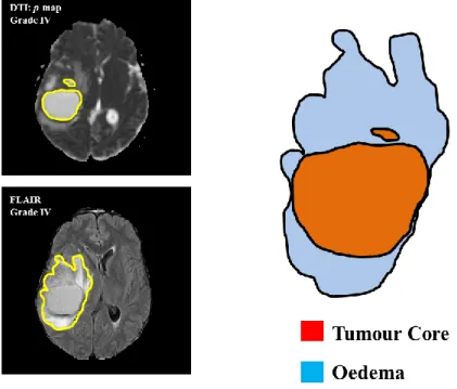
Figure 2-15 Brain tumour tissues (oedema and core) from the clinical dataset. Left) manual ground truth overlaid separately for each tissue on FLAIR (oedema) and DTI p-map (core) protocols. Right: the schematic illustration of the tissues. ... 27

Figure 2-16 Schematic illustration of the regions which are used for evaluation of the segmentation, i.e. Dice score, PPV and sensitivity. Red boundaries represent the manual annotation (ground truth) and the blue areas represent the boundaries of the segmented region using the automated methods. ... 31

Figure 3-1 An illustrative overview of neural network concept of non-linear distortion of the input space to make them linearly separable. The network architecture consists of one input layer, one hidden layer and one output layer. The panels are reproduced from (Colah, 2017). ... 44

Figure 3-2 A general 3D illustration of a CNN architecture. It consists of 3D input layer (image), two 3D hidden layers, and 3D output array. The units of the second hidden layer are also illustrated that they are arranged in 3D structure. Inspired and reproduced from (“CS231n Convolutional Neural Networks for Visual Recognition,” 2017) ... 45

Figure 3-3 A max-pooling example with kernel size 2 × 2 and stride 2. ... 47

Figure 3-4 General overview of CNN architecture. ... 48

Figure 3-5 The structure of inception module proposed in (Szegedy et al., 2015). ... 49

Figure 3-6 Deconvolution and unpooling compared to convolution and pooling (Noh et al., 2015). ... 50

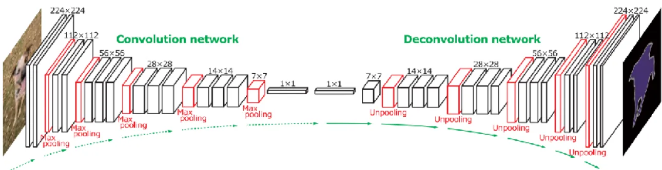
Figure 3-7 The architecture of deconvolutional neural network which was proposed by (Noh et al., 2015). ... 51

Figure 3-8 Architecture of the U-Net which is proposed by (Ronneberger et al., 2015)... 52

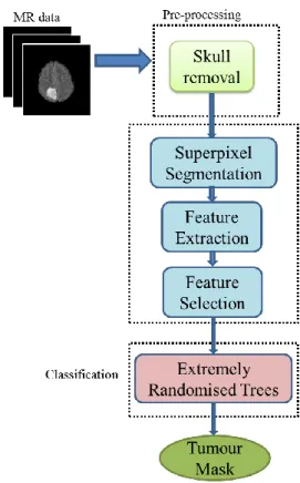
Figure 4-1 The entire workflow of the proposed SP_ERT method ... 61

Figure 4-2 The flowchart of histogram matching and linear normalisation to the range [0, 1]. ... 62

Figure 4-3 Image patch types for local image calculations. a) Fixed-size windows b) homogenous patches with flexible boundaries. The bottom row is the zoomed-in view of the upper row. ... 63

Figure 4-4 Pixel-wise and patch-based calculations schemes. a) pixel-wise, b) patch-based.64 Figure 4-5 Clustering the homogenous pixels to one SP, initialling from a regular grid to the final homogenous superpixel. It should be noted that the centre of the SP may change in each iteration. ... 65 Figure 4-6 Illustration of distance in the SLIC-based superpixel algorithm. SPi presents the

(12)

X

in the search area. The dashed square is the restricted search area around the desired pixel, Pi.

... 66 Figure 4-7 Superpixel segmentation for one slice of the MRI image different compactness factors: a) original MRI FLAIR image with a Grade II tumour, b) superpixel segmentation with m = 0 and S = 10, c) superpixel segmentation with m = 0.2 and S = 10, d) superpixel segmentation with m = 0.5 and S = 10. ... 67 Figure 4-8 Superpixel segmentation for one slice of the MRI image with different window sizes: a) original MRI FLAIR image with a Grade II tumour, b) superpixel segmentation with

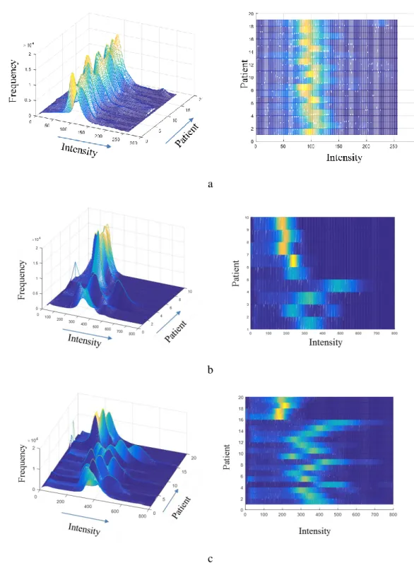
S = 10 (initial grids 10 x 10) and m = 0.2, c) superpixel segmentation with S = 20 (initial grids 20 x 20) and m = 0.2. ... 67 Figure 4-9 Set of Gabor filters which are used for texton feature extraction with different parameters. a) similar sinusoid wavelengths and different sizes and directions, b) similar directions and different sizes and sinusoid wavelengths a) similar sizes and different sinusoid wavelengths and directions, d) 3D representation of Gabor kernels with different sinusoid wavelengths... 72 Figure 4-10 Filter responses obtained by convolving the image with the Gabor kernels in the filter bank separately for different size, direction and sinusoid wavelengths. ... 73 Figure 4-11 Example of calculating texton IDs for normal brain and tumour. The plots present the average texton histogram of the superpixels inside each region, i.e. tumour and normal brain. It should be noted that the IDs are sorted based on the initial k-means cluster points. This is an illustration example and later the clusters will be sorted ascendingly based on the average intensity value of the clusters. ... 74 Figure 4-12 The flowchart of extracting fractal features from a grade III glioma. ... 75 Figure 4-13 An example of fractal analysis applied to a Grade III glioma to generate superpixel based fractal feature maps: a) FLAIR image with the ground truth of oedema, b) area, c) mean intensity, d) fractal dimension. ... 76 Figure 4-14 Fractal dimension vs. mean intensity for healthy and tumour superpixels calculated from one FLAIR MRI data with Grade IV glioma. ... 76 Figure 4-15 FLAIR images with different tumour grades in upper row and their ground-truth manual segmentation of the FLAIR hyperintensity in the lower row. Tumour grades are: a) Grade II b) Grade III and c) Grade IV ... 81 Figure 4-16 FLAIR MRI image histograms for: a) the clinical data original histograms (19 patients), b) BRATS 2013 LGG original histograms (10 patients), c) BRATS 2013 HGG original histogram (20 patients). HGG and LGG are separated for better illustration of the histogram plots. ... 83 Figure 4-17 Comparison of accuracy and superpixel noise for superpixels with S = 6 and different m values in the range [0, 0.45] with the step 0.05. ... 86

(13)

XI

Figure 4-18 Superpixel segmentation with S = 10 and different compactness factors; m = [0.0, 0.5, 0.1, 0.15, 0.2, 0.25, 0.3, 0.4, 0.5, 0.7, and 1.0]. The upper left image is the original FLAIR overlaid with the tumour ground truth, which is the close-up of Figure 4-7. ... 87 Figure 4-19 SP segmentation with different iterations; i.e. Itr = [0, 1, 2, 5, 10]. ... 88 Figure 4-20 Superpixel label difference between iterations for three sample cases and the average of all the cases with S = 6 and m = 0.2. ... 89 Figure 4-21 Comparison of classification accuracy of superpixels on the testing dataset by using different combination of the features (e.g. all features without textons, textons only and all features including textons). ... 90 Figure 4-22 Effect of number of threshold levels on the classification accuracy for Grades II, III, and IV. Adding more threshold levels than nt = 3 does not affect the accuracy. ... 91

Figure 4-23 Comparison of Dice Score overlap measure of SP_SVM vs. SP_ERT for all the clinical patient data (19 scans). Dice score in the vertical axis starts from 0.65 for better illustration. ... 95 Figure 4-24 Comparison between average and standard deviation of Dice score overlap measure for SP_SVM vs. SP_ERT for different tumour grade types II to IV. ... 96 Figure 4-25 Examples of segmentation results overlaid on manual segmentation (green). FLAIR image with tumour Grade II (a1), Grade II (a2), Grade III (a3) and Grade IV (a4); (b1)-(b4) manual segmentation; (c1)-(c4) results using SP_SVM; (d1)-(d4) results using SP_ERT. ... 98 Figure 4-26 Examples of good segmentation results obtained from SP_ERT methods. FLAIR image with tumour Grade II (a1), Grade III (a2), Grade IV (a3); (b1)-(b3) manual segmentation; (c1)-(c3) results using SP_SVM; (d1)-(d3) results using SP_ERT. Most of the false positive superpixels from SP_SVM (e.g. (c1) and (c3)) can be effectively eliminated using SP_ERT; while some tumour superpixels which are wrongly classified to the normal brain tissues by using SP_SVM (e.g.(c2)) can be correctly classified as tumour by using the SP_ERT. ... 99 Figure 4-27 The 3D graphical representationof the segmented tumours in Figure 4-25 using SP_SVM (blue) and SP_ERT (red) overlaid on the ground truth (green). ... 100 Figure 4-28 The 3D graphical representationof the segmented tumours in Figure 4-26 using SP_SVM (blue) and SP_ERT (red) overlaid on the ground truth (green). ... 101 Figure 4-29 Examples of segmentation results obtained from SP_ERT methods on BRATS 2013 data. FLAIR image with high grade tumour Case HG-01 (a1), HG-15 (a2); (b1)-(b2) manual segmentation; (c1)-(c2) results using SP_SVM; (d1)-(d2) results using SP_ERT. 104 Figure 4-30 3D graphical representationof the segmented tumours in Figure 4-29 (HG cases) using SP_SVM (blue) and SP_ERT (red) overlaid on the ground truth (green). ... 105

(14)

XII

Figure 4-31 Examples of segmentation results obtained from SP_ERT methods on BRATS 2013 data. FLAIR image with low grade tumour Case LG-04 (a1), LG-11 (a2) and LG-12 (a3); (b1)-(b3) manual segmentation; (c1)-(c3) results using SP_SVM; (d1)-(d3) results using SP_ERT. ... 106 Figure 4-32 3D graphical representationof the segmented tumours in Figure 4-31 (LG cases) using SP_SVM (blue) and SP_ERT (red) overlaid on the ground truth (green). ... 107 Figure 4-33 Comparison of the average and standard deviation of Dice score overlap measures for SP_SVM vs. SP_ERT for all 19 data scans in the clinical dataset and 30 clinical scans in BRATS 2013 dataset. ... 110 Figure 5-1 The workflow of the proposed automated multimodal MRI segmentation method for segmentation of brain tumour tissue subtypes... 116 Figure 5-2 Flowchart of the multimodal normalisation and histogram matching of the MR dataset. ... 118 Figure 5-3 Fixed and flexible 3D volumes for feature extraction. a) fixed size cubic patches;

WVi represents the window of neighbour voxels around voxel Vi . b) supervoxel patches; SVi

represents the supervoxel i with the centre Ci . ... 119

Figure 5-4 Fixed and flexible 3D volumes for feature extraction. a) fixed size cubic patch. B) flexible homogenous patch volume. The dotted circles are the homogeneous voxels related to regions 1 and 2 that are assigned differently in both patch systems. ... 119 Figure 5-5 Initial supervoxel structure calculation based on MR voxel resolution parameters.

Ws and Hs represent initial supervoxel width and height. Rx and Ry relate to spatial resolution

of the voxel in XY plane, and Rz relates to slice thickness. ... 120

Figure 5-6 Iterative SV portioned the volume into 3D homogenous segments. ... 121 Figure 5-7 Supervoxel segmentation of MRI FLAIR for different supervoxel sizes: a) original image, b) large supervoxel size (30 × 30 × 11), c) small supervoxel size (15 × 15 × 5). .... 122 Figure 5-8 Schematic illustration of the distances for multimodal supervoxel segmentation from protocols: 1 and N. The distances are calculated for the voxel V (yellow point) from two adjacent supervoxels with centre C1 (blue region) and C2 (red region). IVoxel,Pi and ICk,Pi

represents the intensity of V and Ck in protocol i. DV,Ck;P_i is the total intensity distance between

voxel V and Ck in protocol i. ... 123

Figure 5-9 Framework of multimodal supervoxel segmentation. ... 124 Figure 5-10 An example of using a multimodal approach to improve supervoxel boundaries by finding the edges which appear weak in one modality (blue ovals), but are apparent in the other modality (red ovals). (a) Upper image: FLAIR image overlaid by multimodal supervoxel segmentation, lower image: p map overlaid by the same multimodal supervoxel segmentation. (b) Close up of the region surrounded by the yellow box for both image modalities, (c) Close up of the region surrounded by the red box for both image modalities. ... 125

(15)

XIII

Figure 5-11 One comparison example of tumour core supervoxel segmentation (SV) using single modality and multimodal MRI approaches. (a) FLAIR, (b): overlay of the corresponding supervoxels calculated using single modality (FLAIR), (c): zoomed-in of (b) on tumour area (to show the details of the SV boundaries) and overlay of tumour core (ground truth from manual delineation shown in red); (d): protocol p-map, (e): Supervoxels calculated using single imaging modal (FLAIR) overlaid on image protocol p, (f): zoomed-in view of (e) on tumour area and overlay of tumour core (red). (g): protocol p, (h): Supervoxels calculated using multimodal (FLAIR, T1-contrast, T2-weighted, p and q-maps) overlaid on image protocol p-map. (i): zoomed-in of (h) on tumour area and overlay of tumour core (red). The boundaries surrounded by black ellipses in (f) and (i) highlighting the improvement of supervoxel boundary alignment with that of the tumour core using the proposed multimodal SV method. The supervoxels are initially sized 15 × 15 × 5 with m = 0.2 compactness. .... 126 Figure 5-12 Gabor filter orientation and the corresponding angles, i.e. θ and ψ. a) orientation axes illustration, b) a 3D sample for central frequency F, and angles θ and ψ. The blue and red parts correspond to the positive and negative values of Gabor filter, respectively. ... 127 Figure 5-13 3D Gabor filters with different frequencies from various angle views. The blue and red parts correspond to the positive and negative values of Gabor filter, respectively. a) λ = 1.2, b) λ = 1.0, c) λ = 0.8. ... 128 Figure 5-14 a) Example of Gabor filter bank with different filter size and directions and their responses. a) Original FLAIR image, b) Gabor filters with different filter size and directions: rows are corresponding to different filter sizes: [0.3, 0.6, 0.9, 1.2, 1.5] and columns represent different directions: [0o_{, 45}o_{, 90}o_{, 135}o_{] c) the corresponding filter responses obtained by} convolving the filters (b) with the original image (a). ... 129 Figure 5-15 Texton ID histogram for tumour and normal brain. Average of the texton histogram of the regions inside the corresponding regions. ... 131 Figure 5-16 Effect of number of trees on RF classification accuracy with different depths. ... 135 Figure 5-17 Effect of tree depth on RF classification accuracy with different numbers of trees. ... 135 Figure 5-18 Summary of the classification results for supervoxels from Single modality (FLAIR), multimodal C-MRI (FLAIR, T1-contrast and T2-weighted) and C-MRI+DTI (FLAIR, T1-contrast, T2-weighted, p- and q-maps) on clinical dataset. a) precision, b) sensitivity, c) BER. ... 138 Figure 5-19 Comparison example of segmentation of complete tumours using MRI and C-MRI+DTI for three different cases with grade IV tumours. a1-a3) FLAIR image (a1: case

(16)

XIV

37227, a2: case 37230, and a3: case 37256), b1-b3) manual segmentation c1-c2) segmentation using C-MRI d1-d3) segmentation using C-MRI+DTI. ... 140 Figure 5-20 The 3D graphical representation of the complete tumour surfaces from the correponding cases in Figure 5-19. The segmentation surfaces using MRI (blue) and C-MRI+DTI (red) are overlaid on the ground truth (green). ... 141 Figure 5-21 Segmentation results for the core of tumours using C-MRI and C-MRI+DTI for three different cases with grade IV tumours. a1-a3) FLAIR image (a1: case 37227, a2: case 37230, and a3: case 37256), b1-b3) manual segmentation c1-c2) segmentation using C-MRI d1-d3) segmentation using C-MRI+DTI... 142 Figure 5-22 The 3D graphical representation of the tumour core surfaces from the correponding cases in Figure 5-21. The segmentation surfaces using MRI (blue) and C-MRI+DTI (red) are overlaid on ground truth (green). ... 143 Figure 5-23 Segmentation results overlaid on the ground truth (complete tumour including oedema and core), using single (FLAIR) and multi-protocol (C-MRI including FLAIR, T1-weighted, T1-contrast and T2-weighted); a1)-a3) FLAIR image, b1)-b3) manual segmentation (green) c1)-c3) segmentation using FLAIR (red) d1)-d3) segmentation using conventional MRI (blue). ... 147 Figure 5-24 The 3D graphical representation of the complete tumour surfaces from the correponding cases in Figure 5-23. The segmentation surfaces using single-protocol (red) and multi-protocol (blue) are overlaid on ground truth (green). ... 148 Figure 5-25 Segmentation results overlaid on the ground truth (tumour core), using single (FLAIR) and multi-protocol (C-MRI including FLAIR, T1, T1-contrast and T2-weighted) for the same three cases shown Figure 5-23. a1)-a3) FLAIR image, b1)-b3) manual segmentation (green) c1)-c3) segmentation using FLAIR (red) d1)-d3) segmentation using conventional MRI (blue)). ... 149 Figure 5-26 The 3D graphical representation of the tumour core surfaces from the correponding cases in Figure 5-25. The segmentation surfaces using single-protocol (red) and multi-protocol (blue) are overlaid on ground truth (green). ... 150 Figure 5-27 Average classification results for supervoxels from single modality (FLAIR) and multimodal C-MRI of the BRATS 2013 dataset. a) precision, b) sensitivity, c) BER. ... 151 Figure 5-28 Comparison results for Dice overlap ratio between manual annotation and the automated segmentation using: a) single modality (FLAIR), multimodal MRI, and C-MRI+DTI of the clinical dataset, b) single modality (FLAIR) and multimodal C-MRI of BRATS 2013 dataset. ... 154 Figure 5-29 Overall comparison tumour segmentation. A) FLAIR image, B) manual segmentation of the core (yellow region) and oedema (red region) C) segmentation using conventional MRI, D) segmentation using MRI+DTI, E) comparison of both methods

(17)

C-XV

MRI (red), plus DTI (blue) and manual (green) segmentation for core (zoomed in), F) comparison of both methods C-MRI (red), C-MRI+DTI (blue) and manual (green) segmentation for oedema (zoomed in). ... 155 Figure 5-30 Comparison between single-modal and multimodal segmentation of the core. a-c) FLAIR, d-f) T1-contrast. Green: manual ground truth, red: single-modal, blue: multimodal. ... 156 Figure 6-1 Schematic architectures of the convolutional networks. a) standard CNN takes fixed size input in FC layer, b) standard FCN (classification) takes input with any size and the output is the feature vector or classification value, c) modified FCN for dense pixel segmentation takes input with any size and produces output with the same size. ... 163 Figure 6-2 Schematic illustration of how different resolution feature information are considering from different depth of layers. ... 165 Figure 6-3 The detailed architecture of the FCN used for segmentation of brain tumour in multimodal MRI... 167 Figure 6-4 Comparison of the multimodal MRI segmentation output of the FCN-8s network with the ground truth. ... 168 Figure 6-5 The overall flowchart of the hybrid method which uses hand-designed and machine-learned features for automatic brain tumour segmentation in MRI images. ... 169 Figure 6-6 The score maps are extracted from the deconvolution layer from the FCN... 170 Figure 6-7 The FCN-based score maps generated from the multimodal MRI images.. ... 171 Figure 6-8 The texton maps generated from the M-MRI images. The figures are shown for challenge case number HG-0309 (ID: 17604) and slice 59. a-c) Original MRI: a) FLAIR, b) T1-contrast, and c) T2-weighted. d-f) texton feature map extracted separately from the protocols: d) FLAIR, e) T1-contrast, and f) T2-weighted. ... 172 Figure 6-9 The connectivity of the adjacent pixels from the histogram of the texton IDs in a 5 × 5 neighbourhood of the centre pixel. The texton clusters are integers in the range [1, 6]. The texton IDs outside the neighbourhood are not counted. This is a simplified example to illustrate the procedure of texton histogram feature extraction from the pixel neighbourhood. The texton histogram values are zero for IDs from 6 to 16 in this example. ... 174 Figure 6-10 (Upper row) T1-contrast, FCN-based score map of enhancing core, texton map of T1-contrast, and ground truth; (middle row) the corresponding close up of the upper row images and two different pixels with GT labels: enhancing (black square) and necrosis (red square); (lower row) the features extracted for the corresponding pixels including FCN-based score of “enhancing”, and connected textons ID histogram in a 5 × 5 neighbourhood around the centre pixel. ... 174 Figure 6-11 (Upper row) FLAIR, FCN-based score map of “oedema”, texton map of FLAIR, and ground truth; (middle row) the corresponding close up of the upper row images and two

(18)

XVI

different pixels with GT labels: oedema (black square) and normal brain (red square); (lower row) the features extracted for the corresponding pixels including FCN-based score of “oedema”, and connected textons ID histogram in a 5 × 5 neighbourhood around the centre pixel. ... 175 Figure 6-12 The detailed of feature vector generation for the hybrid method. Machine based features from FCN are extracted based on pixel and the hand-designed texton features extracted from the neighbourhood around the pixel and considers the local dependencies. 176 Figure 6-13 Segmentation results for some cases of BRATS 2013 challenge dataset. ... 180 Figure 6-14 Segmentation results for some cases of BRATS 2013 challenge dataset. a) the original FLAIR images, b) T1-weighted-contrast, c) segmentation mask of FCN_RF overlaid on the FLAIR image. Oedema: green, necrosis: blue, enhancing tumour: red. ... 181 Figure 6-15 Segmentation results for some cases of the BRATS 2013 challenge dataset. a) the original FLAIR images, b) T1-weighted-contrast, c) segmentation mask of the FCN_Texton_RF method overlaid on the FLAIR image. ... 183 Figure 6-16 Comparison of DSC (average and standard deviation) for the three experiments separated for whole, tumour core and enhancing tumour. ... 184 Figure 6-17 Comparison of PPV (average and standard deviation) for the three experiments separated for whole, tumour core and enhancing tumour. ... 185 Figure 6-18 Comparison of Sensitivity (average and standard deviation) for the three experiments separated for whole, tumour core and enhancing tumour... 185 Figure 6-19 Segmentation masks for some validation datasets, using the proposed method. The case names and the slice number are mentioned on the top of the images. Upper row) FLAIR images, middle row) T1-contrast images, lower row) segmentation masks and labels using the proposed method. ... 187 Figure 6-20 Comparison of DSC overlap measure with top ranked methods which used BRATS 2013 challenge dataset. ... 190 Figure 6-21 Comparison of PPV measure with top ranked methods which used BRATS 2013 challenge dataset. ... 191 Figure 6-22 Comparison of sensitivity measure with top ranked methods which used BRATS 2013 challenge dataset. ... 192 Figure 6-23 An example of failure of the proposed FCN_Texton_RF method for segmentation of tumour core in the case HG-0307 of BRATS 2013 challenge dataset. ... 195

(19)

XVII

List of Tables

Table 2-1 T1 and T2 times for the brain tissues at magnetic field of B0 = 1 Tesla. ... 12

Table 2-2 The classification evaluation categories. ... 30 Table 3-1 Summary of MICCAI-BRATS results for the publications related to the literature review. The evaluation dataset and Dice scores for the tumour part are provided. The research papers are sorted based on the publication year. ... 55 Table 4-1 Total number of features calculated from an MRI FLAIR image ... 77 Table 4-2 Dice overlap comparison results for the BRATS data with histogram normalisation and without histogram normalisation (but normalising the feature ranges, so it is called “partial normalisation” in this table). ... 84 Table 4-3 Examples of the impact of different initial superpixel side sizes, S, on the segmentation accuracy of the tumour in FLAIR images with compactness factor m = 0.2 ... 88 Table 4-4 Impact of the number of trees on ERT classifier accuracy and training time... 92 Table 4-5 Comparison of feature selection techniques. The accuracy of ERT classifier after feature selection is considered as evaluating the efficiency of the selected feature subsets. . 92 Table 4-6 Comparison evaluation on superpixel classification in SP_SVM and SP_ERT, respectively, on the 5 features selected using mRMR. The classification is performed for tumour including oedema and active tumour core versus normal brain tissue. (BER is balanced error rate). ... 94 Table 4-7 Statistical parameters of the Wilcoxon signed-rank test ... 96 Table 4-8 Comparison evaluation on superpixel classification using SP_SVM and SP_ERT classifier, respectively, on the BRATS 2013 dataset using 5 features selected by mRMR. The classification is performed for tumour including oedema and active tumour core versus normal brain tissue (BER is balanced error rate). ... 102 Table 4-9 Comparison results for Dice overlap ratio between manual annotation and the automated segmentation using SP_SVM and SP_ERT for BRATS 2013 dataset (30 scans). ... 103 Table 4-10 Comparison with other related methods using BRATS dataset (MICCAI 2013). Note: the proposed SP_ERT method and Reza et al. (Reza and Iftekharuddin, 2013) are performed on BRATS clinical training data and the other work (Tustison et al. (Tustison et al., 2013)) is performed on BRATS challenge data. ... 111 Table 5-1 Summary of the features and their corresponding numbers which are used for the proposed learning based method. ... 130 Table 5-2 Ranking of the features from each individual protocol in different multimodal experiments on the clinical dataset, based on their repetition in nodes of the forests of a RF with Ntree = 50 number of trees and Dtree = 15. ... 136

(20)

XVIII

Table 5-3 Classification results (average values over all the LOO-CV) for superpixels using single MRI protocol (FLAIR). ... 137 Table 5-4 Classification results (average values over all the LOO-CV) for superpixels using conventional MRI protocols (FLAIR, T1-contrast, T2-weighted). ... 137 Table 5-5 Classification results (average values over all the LOO-CV) for superpixels using MRI conventional protocols plus DTI (FLAIR, T1-contrast, T2-weighted, p and q) ... 137 Table 5-6 Dice score comparison for the segmentation of tumour core, oedema and complete tumour in clinical dataset using single protocol (FLAIR), C-MRI (FLAIR, T1-contrast, T2-weighted) and C-MRI+DTI (FLAIR, T1-contrast, T2-weighted, p and q-maps). ... 139 Table 5-7 Classification results for supervoxels from FLAIR protocols of BRATS 2013 dataset. ... 144 Table 5-8 Classification results for superpixels from MRI Multi protocols (FLAIR, T1, T1-contrast and T2-weighted) of BRATS 2013 dataset. ... 145 Table 5-9 Comparison results for DSC between manual annotation and the automated segmentation using a single protocol (FLAIR) and multi-protocol (FLAIR, weighted, T1-contrast and T2-weighted) of BRATS 2013. ... 146 Table 5-10 Wilcoxon signed-ranks test statistical parameters results for the segmentation overlap measure of DSC and the classification measures using FLAIR only, MRI, and C-MRI+DTI) on the clinical dataset (11 subjects). ... 152 Table 5-11 Wilcoxon signed-ranks test statistical parameters results for the segmentation overlap measure of DSC and the classification measures using FLAIR only, and C-MRI on BRATS dataset (30 subjects). ... 152 Table 5-12 Wilcoxon signed-ranks test statistical parameters results for the segmentation overlap measure of DSC and the classification measures using FLAIR only, and C-MRI, on both the clinical and BRATS 2013 dataset (41 subjects). ... 153 Table 5-13 Dice score comparison of the proposed multimodal SV_RF with other methods which used BRATS 2013 training dataset (MICCAI 2012 and 2013). ... 157 Table 6-1 Details of the features which are used in the proposed method. ... 176 Table 6-2 Segmentation results per case for BRATS 2013 challenge dataset using FCN only, evaluated by the VSD website system. ... 179 Table 6-3 Segmentation results per case for the BRATS 2013 challenge dataset using FCN_RF, evaluated by the VSD website system. ... 181 Table 6-4 Segmentation results per case for the BRATS 2013 challenge dataset using FCN_Texton_RF, evaluated by the VSD website system. ... 183 Table 6-5 Segmentation results for the BRATS 2017 validation dataset, which was provided by CBICA portal. The results are the overall average and standard deviation of 46 patient cases. ... 186

(21)

XIX

Table 6-6 Segmentation results for BRATS 2013 challenge dataset which is evaluated by VSD website. Comparison with other works which used BRATS 2013 challenge dataset and are top ranked. The values which are presented in parentheses in the third row are the current ranking of the proposed method in each section, on VSD scoreboard (Appendix 2). ... 189

(22)

XX

List of Abbreviations

2D Two dimensional

3D Three dimensional

AlexNet The CNN proposed in (Krizhevsky et al., 2012)

ANN Artificial neural networks

BER Balanced error rate

BFC Bias field correction

BRATS Multimodal brain tumour segmentation challenge

BraTumIA Brain tumour image analysis

CART Classification and regression trees

C-MRI Conventional magnetic resonance imaging

CNN Convolutional neural networks

CONV Convolutional layer

CONV_ReLU Convolutional layer + rectified linear unit

CRF Conditional random fields

CSF Cerebral spinal cord

CT Computed tomography

DeCONV Deconvolutional layer

DL Deep learning

DSC Dice similarity score

DTI Diffusion tensor imaging

DWI Diffusion weighted imaging

ERT Extremely randomised trees

FC Fully connected layer

FCBF Fast correlation-based filter

FCM Fuzzy c-means

FCN Fully convolutional neural network

FCN_RF Fully convolutional network and random forests

FCN_Texton_RF Fully convolutional network, texton, and random forests

FLAIR Fluid attenuated inversion recovery

FN False negative

FP False positive

GM Grey matter

GoogleNet The CNN proposed by Google (Szegedy et al., 2015)

HGG High grade gliomas

IID Independent and identically distributed

ILSVRC ImageNet Large-Scale Visual Recognition Challenge

IR Inversion time

LeNet The CNN proposed by LeCun et al. (LeCun et al., 1998)

LGG Low grade gliomas

LOO-CV Leave-one-out cross validation

MAP Maximum a posteriori

MICCAI Medical Image Computing and Computer Assisted Intervention

MIUA Medical Image Understanding and Analysis

(23)

XXI

MR Magnetic resonance

MRF Markov random fields

MRI Magnetic resonance imaging

mRMR Minimum redundancy maximum relevance

PD Proton density

POOL Pooling layer

ReliefF Feature selection method proposed in (Kononenko, 1994)

ReLU Rectified linear unit

ResNet Residual networks

RF Random forests

ROI Region of interest

SBMLR Sparse logistic regression with Bayesian regularisation

SFTA Segmentation based fractal texture analysis

SGD Stochastic gradient descent

SKIP Skip layer

SLIC Simple linear iterative clustering

SLogReg Sparse logistic regression

SP Superpixel

SP_ERT Superpixel and extremely randomised trees

SP_SVM Superpixel and support vector machines

SPEC Spectral feature selection

SPM Statistical parametric mapping

STD Standard deviation

SV Supervoxel

SVM Support vector machines

TE Echo time

TN True negative

TP True positive

TR Repetition time

U-Net The CNN proposed in (Ronneberger et al., 2015)

VGGNet The CNN proposed in (Simonyan and Zisserman, 2014)

VSD Virtual skeleton database

WM White matter

(24)

1

Chapter 1

1 Introduction

1.1 Problem statement

The incidence rate of brain related tumours in the United Kingdom has been estimated to be approximately 11,000 cases in 2014 from which 46% were primary brain tumour (“Cancer Research UK,” n.d.). Although the relative occurrence of brain cancer is low compared to other types of adult cancers1_{, they affect significantly the lives of the people more than other} types of cancer (“Cancer registration statistics, England Statistical bulletins - Office for National Statistics,” n.d.).

Brain tumours can arise from abnormal growth of the cells inside the brain or can develop from cells that have spread to the brain from a cancer elsewhere. There are a wide variety of brain tumour types that are classified according to their cell of origin. The primary tumours are those started within the brain. The majority of primary brain tumours originate from glial cells (termed glioma) and are classified by their histopathological appearances using the World Health Organisation (WHO) system into low grade glioma (LGG) and high grade glioma (HGG).

Medical imaging modalities are used for detection and assessment of tumours. Among different imaging modalities, magnetic resonance imaging (MRI) is one of the most widely used modalities for clinical diagnosis, treatment selection, prognosis and to aid surgery and radiotherapy planning (Fink et al., 2015). Due to the multimodal nature of MRI, which will be explained in Chapter 2, there are a range of image types and contrasts that enable a subtle radiological assessment of tumour type.

Delineation of the tumour boundary and assessment of tumour size are needed for patient management in terms of treatment planning and monitoring treatment response (Eisele et al., 2016), and current guidelines incorporate the use of conventional MR images (C-MRI) (Niyazi

et al., 2016; Wen et al., 2010). C-MRI can also be useful to help define the target volumes for radiotherapy planning of high-grade gliomas (Aslian et al., 2013; Niyazi et al., 2016). Tumour assessment requires accurate full 3D volume measurement of the tumour which is obtained by manually drawing around the region of interest (ROI). Manual segmentation around tumour margins on a slice-by-slice basis is time-consuming and can take 12 minutes or more per

1_{The percentage of brain tumour was 3% of total cancer cases in the UK in 2014 (“Cancer Research}

(25)

2

tumour, with semi-automatic methods taking 3 to 5 minutes (Aslian et al., 2013; Odland et al., 2015). Furthermore, a human has limitations in detecting the visual features of the image which increases the risk of human error in manual segmentation. Therefore, an automated segmentation that is not subject to operator subjectivity may be beneficial (Aslian et al., 2013), especially for the large-sized MRI data.

1.2 Motivations

Using computer-aided procedures for medical diagnosis and treatment tasks is a fast-growing field of research nowadays. Computer based analysis and measurements of medical images help the clinicians to obtain the measures and identifications faster and more accurate. Medical image analysis plays an important role in clinical procedures related to brain tumours by providing clinicians with automated (or semi-automated) computing tools to help them in diagnosis and treatment tasks. For brain tumours, accurate segmentation may aid the fast (approximately 5 minutes for each patient image) and objective measurement of tumour volume and also find patient-specific features that aid diagnosis and treatment planning (Gordillo et al., 2013). However, automated segmentation of brain tumours is a very challenging task due to their high variation in size, shape and appearance (e.g. image uniformity and texture) (Patel and Tse, 2004).

Many segmentation methods have been proposed for brain tumour segmentation which will be reviewed in Chapter 3. Despite much effort being devoted to the segmentation problem, brain tumour segmentation remains an ongoing research topic.

Most of the existing studies on brain tumour segmentation are performed on conventional MRI protocols, which are based on qualitative image intensities. Considering the advanced MR acquisition protocols, i.e. diffusion tensor imaging (DTI), in the segmentation process may provide more useful information to increase the accuracy. The isotropic (p) and anisotropic (q) diffusion components derived from DTI (Peña et al., 2006) provide parameters that relate to the microstructure of the brain tissues. The hypothesis of combining DTI and C-MRI is that they may provide quantitative features that increase the classification accuracy and improve tumour segmentation results. Furthermore, many LGG tumours do not show contrast enhancement hence conventional images are used to define the tumour extent and volume. A study has shown that LGG volume and growth rate can be used to assess whether patients are at risk with tumours likely to undergo an early malignant transformation (Rees et al., 2009). Using advanced MR techniques may tackle this problem which should be investigated by combining and comparing to the conventional MR protocols.

(26)

3

Learning based segmentation techniques require a lot of training data which increases the complexity and computing time and memory. Since most segmentation algorithms are based on pixel classification in single/multiple images, in the case of multimodal MR images, the large number of voxels to be processed will significantly increase computational burden. Partitioning the images into small subregions with homogenous properties will decrease the data dimensionality by decreasing the feature space.

Due to the recent advances in deep neural networks (DNNs) in recognition of the patterns in the images, most of the recent tumour segmentations have focused on deep learning methods. Amongst DNNs, the methods based on deep convolutional neural networks (CNNs) has recently provided the best performance in the computer vision and brain tumour segmentation competitions. The CNNs can learn the image patterns in different levels of hierarchy and resolutions. However, the CNNs are, in fact, classifiers which have been used for whole-image classification (Krizhevsky et al., 2012) or local tasks such as object detection (Sermanet et al., 2013). For the task of image segmentation in the pixel resolution level, CNNs have been modified by adding pre- or post-processing blocks (Hariharan et al., 2014). However, these approaches have limitations of lacking a whole end-to-end learning, since the additional blocks are independent from CNN training process. Recently, fully convolutional networks (FCN) have been suggested for dense (i.e. per-pixel) classification with the advantage of end-to-end learning (Long et al., 2015), without requiring those additional blocks in CNN-based approaches. FCN can take an input image with any size, yielding the hierarchy of the features, and provide dense prediction with input-matching size. Despite the advantage of dense pixel classification, FCN-based methods still have limitations of considering the local dependencies in higher resolution (pixel) level. The loss of data, which occurs in the pooling layers, results in coarse segmentation. This limitation will be addressed in this thesis by incorporating high resolution hand-designed textural features which consider local dependencies of the pixel. Texton feature maps (Arbelaez et al., 2011) provides significant information on multi-resolution image patterns in both spatial and frequency domains. This is an inspiration to combine texton features to a partially end-to-end learning process in order to improve the segmentation. The term “partially” is considered for end-to-end learning since the proposed method in this thesis is trained on a pretrained model, which will be discussed later in Chapter 6.

Most classification-based techniques have proposed and/or optimised the hand-designed features, while deep learning based methods automatically learn the features from the images. A hypothesis is that combining both hand-designed and machine-learned features encodes global information and local dependencies into feature representation, which results in more accurate segmentation.

(27)

4

1.3 Aims and objectives

The aim of this research is to develop automatic image processing techniques to accurately detect and segment the brain tumour tissue subtypes from multimodal MR images, including conventional and advanced acquisition techniques. This thesis will focus on statistical learning based medical image segmentation using hand-designed and machine-learned features. To achieve this aim, the following objectives are considered:

 Developing and validating an automated method for a single MRI modality to segment the abnormal tumour part from the normal brain tissues.

 Building a generic framework which combine both C-MRI and DTI to incorporate information from multimodal clinical MRI images. Since each imaging protocol contains specific features from the tissues, merging them together may provide more accurate segmentation of tumour tissue subtypes.

 Exploring a new feature representation which combines hand-designed features (e.g. texton) considering local dependencies, and machine-learned features (from FCN) which provides better object localisation, for accurate segmentation of brain tumours.

 Evaluating the proposed algorithms by conducting experiments on different datasets, i.e. a clinical dataset, which are acquired from St George’s Hospital Trust London, and a publicly available dataset of Multimodal Brain Tumour Image Segmentation Benchmark (BRATS) (“BRATS :: The Virtual Skeleton Database Project,” n.d.; Kistler et al., 2013; Menze et al., 2015).

1.4 Contributions

The main contribution of this thesis can be summarised as follows

 Developing a fully-automated learning based method for detection and segmentation of the abnormal tissue associated with brain tumours as defined by the T2 hyperintensity from Fluid Attenuated Inversion Recovery (FLAIR) MRI as a single protocol (Chapter 4). The previous methods have used multi-protocols to perform the automatic segmentation (Davy

et al., 2014; Havaei et al., 2017), while this thesis introduced a method that uses one single protocol to segment the tumour. However, this single-modality method is suitable for segmentation of the whole tumour. Further segmentation of the tumour tissue subtypes requires more protocols, which will be discussed later chapters.

 Incorporating advanced MR acquisition protocols, i.e. DTI alongside with C-MRI for accurate segmentation of brain tumours by fusing the image intensities and features into a unified framework. The isotropic (p) and anisotropic (q) diffusion components derived

(28)

5

from DTI (Peña et al., 2006), which are related to the microscopic structures of the tissues, provide more information about tumour structure which improves the multi-class tumour segmentation (Chapter 5). Using DTI protocols in segmentation of brain tumour via superpixel analysis and random forest classification is one of the novelties of this thesis.

 Proposing a unified framework for partitioning the multimodal MR images into small clusters (e.g. supervoxels) by incorporating the MR volumetric characteristics, i.e. voxel dimension and slice thickness. The previous methods (Su et al., 2013) have used the pixels in the raw slices without considering the voxel characteristics. The information from multimodal images is combined to produce supervoxel boundaries across multiple image protocols. The advantage of the supervoxel based method is that the required computation for classification in the new feature space can be significantly reduced (Chapter 5).

 Proposing the histogram of texton descriptors particularly for superpixels/supervoxels using Gabor filters as one of the main features, since they are able to distinguish various textural patterns in the image. The previous methods based on superpixel histogram (Fulkerson et al., 2009) have not used texton at a superpixel level. The previous texton-based method (Yu et al., 2012) has used Gaussian filter banks. The related works, which used the histogram of Gabor filter responses as the representation of the features (Yi and Su, 2014), suggested using fixed-sized non-overlapping blocks of the images. In this thesis, flexible superpixel patches are used instead of the fixed blocks. Textons were calculated using a set of Gabor filters with different sizes and orientations, to increase the performance for classification of brain tumour superpixels (Chapter 4) and supervoxels (Chapter 5). Also, another novelty of texton features in Chapter 5 is using 3D Gabor filter banks for MRI volumetric datasets.

 Proposing a novel fully automatic learning based segmentation method, by applying hand-designed and machine-learned features to the state-of-the-art random forest (RF) classifier. The machine-learned FCN based features detect the coarse region of the tumour while the hand-designed texton descriptors consider the spatial features and local dependencies to improve the segmentation accuracy (Chapter 6). The previous Gabor-based CNN methods either fused the Gabor filters to the architecture of CNN (Luan et al., 2017) or used the feature maps from the Gabor filters as an input to the network (Yao et al., 2016). In this thesis, the Gabor-based textons features are considered as a neighbourhood system in the pixel level to compensate the loss of information that occurs in the pooling layers of the FCN.

The current research has resulted in 5 papers (one published journal, one journal under revision, one magazine, and two conferences) that are listed in Appendix 1.

(29)

6

1.5 Thesis Structure

Chapter 2 describes the clinical background of the brain tumour segmentation in MRI images. The focus will be on MRI acquisition technique which is common for brain tumour clinical tasks. Different MRI modalities will be explained. The datasets which are used for evaluation will be described followed by the evaluation protocols for brain tumour segmentation. Chapter 3 presents the technical literature review on brain tumour segmentation using different MRI modalities. The chapter will also analyse specifically the related research work which use the most common publicly available MRI dataset specialised for the field of brain tumour segmentation, i.e. Brain Tumor Image Segmentation Benchmark (BRATS), and the relevant challenge, i.e. Medical Image Computing and Computer Assisted Intervention (MICCAI). Chapter 4 investigates single modality learning based brain tumour segmentation using hand-designed features. FLAIR is used to detect the tumour since it is the most common clinically acquired protocol to detect and segment complete tumour structure. The texton map will be generated from the FLAIR image, from which texton histogram is calculated for each superpixel and will then be used as one of the main features. Extremely randomised trees (ERT) classifier will be investigated which is a powerful classifier that can deal with high dimensional features and large-sized unbalanced data.

Chapter 5 investigates multimodality brain tumour segmentation in three-dimensional space using hand-designed features. The texton histogram and feature maps are calculated for the supervoxels from the 3D image volume. The segmentation of brain tumour is developed further to its tissue subtypes, i.e. core and oedema, by defining multi-object classification problem. Effect of advanced MR imaging techniques (DTI) is also investigated and compared to conventional MRI protocols.

Chapter 6 introduces using the combination of hand-designed and machine-learned feature for learning based segmentation of brain tumours. The machine-learned features are extracted from the FCN. The main idea is to overcome the drawbacks of machine-learned features by considering the local dependencies which are obtained by hand-designed textural features. The algorithm is also further extended to the segmentation of more details from the tumour structures, i.e. oedema, necrosis, enhancing and non-enhancing tumour cores. This will also make the method comparable with other state-of-the-art work which are using the public datasets.

Chapter 7 summarises the thesis and provides the discussion and conclusion, and presents the future directions.

(30)

7

Chapter 2

2 Clinical Background

2.1 Introduction

Application of medical imaging for brain tumour diagnosis has developed over the past decades. The aim of brain tumour imaging is to identify the location and size of the tumour. This will help the clinical tasks such as diagnosis, surgical and radiotherapy planning. It is also used to evaluate the treatment results, e.g. follow up study after treatment.

Regarding the developments in MRI systems, they are now widely used for brain tumour patient evaluation tasks (Jenkinson et al., 2007). The advantages of MRI compared to other techniques, such as computed tomography (CT) images can be summarised as: high contrast between the soft tissues, higher resolution than CT, and non-ionising radiation.

MRI sequences are generally classified into “conventional” and “advanced”. Conventional MRI (C-MRI) techniques provide qualitative images of the tissues. Advanced MRI images provide quantitative or semi-quantitative measurements of the brain tissues. In this chapter, firstly the conventional MRI will be introduced followed by its application in brain tumour diagnosis. Then, the advanced MRI techniques on diffusion imaging will be explained.

2.2 Brain Tissues

The brain is the most complex organ of the body and it consists of many parts. The most distinguished parts in MR images are Grey Matter (GM), White Matter (WM) and Cerebrospinal Fluid (CSF). GM is the major component of the brain. It consists of mostly body cells and few myelinated axons. WM contains myelinated axons and glial cells. CSF is a clear fluid exists in ventricular system inside and around the brain and spinal cord.

2.3 Conventional MRI

Magnetic resonance (MR) is defined as the result of interaction between the magnetic moment of a nucleus spin and an external magnetic field. Three types of magnets are used to create the MR signal and are electromagnet, permanent magnet, and superconducting magnet. Superconducting magnets are extensively used in modern MR scanners which can produce very strong fields of up to 8 Tesla. In current clinical application, the strength of 1.5 to 3 Tesla are used.

(31)

8 2.3.1 The Physics behind MRI

MRI utilises the properties of spin to acquire images. The atom elements, i.e. protons, neutrons and electrons, spin around a central axis. Nuclei with an odd mass number (MR active nuclei), such as hydrogen (H1), create a net nonzero spin which acquire a magnetic moment. Their magnetic moment will align their axis of rotation when they are exposed to an external magnetic field.

When no magnetic field is applied to a MR active nuclei, the magnetic moment of the nuclei is oriented in random directions. Therefore, the net magnetic field will be zero. By applying an external magnetic field of B0, the nuclei will align along the flux lines of field.

When a hydrogen nucleus is exposed to an external magnetic field, a secondary spin will be added to its normal spin which is like wobbling around its magnetic moment around B0. This

spin is called “precession” and forces the magnetic moments to have a circular precessional path at precessional frequency speed which is called “Larmor frequency”.

2.3.2 Resonance

Resonance is occurred when a radiofrequency (RF) pulse (“excitation” pulse) is applied at the same energy of precessing hydrogen nuclei at angle of 90 degrees to the field B0. At the

resonance, two phenomena will occur which are energy absorption and phase coherence. In the presence of external magnetic field (B0), the number of spin-up and spin-down nuclei

are equal (Figure 2-1-(a)). The net magnetisation vector (NMV) lies in the transverse (X-Y) plane (90), which is known as “flip angle”. The hydrogen nuclei absorb energy from the RF pulse. This will increase the number of high energy (spin-down) nuclei (Figure 2-1-(b)). The magnitude and duration of the RF pulse affect the magnitude of the flip angle. By increasing the magnetic field B0 the required energy for generating resonance will also increase. It should

be noted that, the Figure 2-1 shows a schematic representation of NMV before and after applying the RF pulse to the MR active nuclei.

Phase coherence occurs at resonance when the magnetic moment of hydrogen is aligned in the same position of the processional route around the magnetic field B0. This is also called

in-phase (coherent). It results in a superimposed magnetic vector in the X-Y plane which is depicted in Figure 2-1-(d) which is called transverse magnetisation.

(32)

9

a b

c d

Figure 2-1 Effect of applying RF pulse when the nuclei is exposed to the external magnetic field. NMV which is related to the spin-up and spin-down nuclei: a) without application of RF pulse, and b) when a RF pulse is applied the number of spin-down (high energy) nuclei increases which results in a NMV. Phase coherence: c) out of phase or incoherent in the absence of RF pulse, and d) in-phase or coherent when applying the RF pulse at Larmor frequency.

2.3.3 MR Signal Generation

To create a MR signal, a strong and constant magnetic field is applied to the target sample or tissue. As explained in Section 2.3.2, resonance produces in-phase magnetisation precessing in the transverse plane. This magnetisation can induce a voltage when it cuts across the receive coil which creates the MR signal. The magnitude of the signal is related to the amount of magnetisation in the transverse plane and the frequency of the signal is equal to Larmor frequency.

After termination of the RF pulse, the nuclei will lose the energy obtained from the RF pulse and the NMV tries to realign with the external magnetic field B0. The magnetisation in

longitudinal plane increases which is known as recovery and has exponential properties. Meanwhile, the magnetisation in the transverse plane decreases exponentially which is known as “decay”. The induced voltage magnitude in the receiver coil will decrease during the decay which is called free induction (FID) signal. The effect of applying RF pulse and creating the FID signal is depicted in Figure 2-2.

(33)

10

Figure 2-2 Effect of applying RF pulse and generating the FID signal, high energy or spin-down (red) and low energy or spin-up (blue).

2.3.4 Relaxation

During the relaxation phase, the hydrogen nuclei will discard the energy that was absorbed when RF was applied. As a result, the NMV returns back to the initial B0 and the magnetic

moments of hydrogen nuclei lose their coherency. The longitudinal magnetisation is recovered by the recovery process which is called T1 recovery. And the transverse magnetisation is decayed by the process T2 decay. Figure 2-3 presents the recovery and decay processes.

a b

Figure 2-3 a) T1 recovery curve which represents exponentially increasing longitudinal magnetisation. T1 recovery is the time taken for 63% of the longitudinal magnetisation (Mz)

to recover b) T2 decay curve which represents the decay of magnetisation in transverse plane (Mxy) after switching off the RF pulse. T2 relaxation is the time taken for 63% of the transverse

magnetisation to be faded.

T1 Recovery

When nuclei release their energy, which is called spin-lattice relaxation, it results in T1 recovery. This leads the magnetic moments of nuclei to recover longitudinal magnetisation.