Universidade de São Paulo
2014-08
Extracting texture features for time series
classification
International Conference on Pattern Recognition, 22nd, 2014, Stockholm.
http://www.producao.usp.br/handle/BDPI/48622
Downloaded from: Biblioteca Digital da Produção Intelectual - BDPI, Universidade de São Paulo
Biblioteca Digital da Produção Intelectual - BDPI
Extracting Texture Features for Time Series
Classification
Vin´ıcius M. A. Souza, Diego F. Silva, Gustavo E. A. P. A. Batista
Instituto de Ciˆencias Matem´aticas e de Computac¸˜ao Universidade de S˜ao Paulo
{vsouza, diegofsilva, gbatista}@icmc.usp.br
Abstract—Time series are present in many pattern recognition applications related to medicine, biology, astronomy, economy, and others. In particular, the classification task has attracted much attention from a large number of researchers. In such a task, empirical researches has shown that the 1-Nearest Neighbor rule with a distance measure in time domain usually performs well in a variety of application domains. However, certain time series features are not evident in time domain. A classical example is the classification of sound, in which representative features are usually present in the frequency domain. For these applications, an alternative representation is necessary. In this work we investigate the use of recurrence plots as data representation for time series classification. This representation has well-defined visual texture patterns and their graphical nature exposes hidden patterns and structural changes in data. Therefore, we propose a method capable of extracting texture features from this graphical representation, and use those features to classify time series data. We use traditional methods such as Grey Level Co-occurrence Matrix and Local Binary Patterns, which have shown good results in texture classification. In a comprehensible experimental evaluation, we show that our method outperforms the state-of-the-art methods for time series classification.
I. INTRODUCTION
Time series are ubiquitous in almost every human activity. Time oriented data are present in many application domains such as medicine, biology, economy, signal processing, among others. Consequently, the analysis of time series data has attracted much attention and effort from several researchers around the world. Time series analysis can be divided in dif-ferent tasks, such as classification, clustering, motif discovery, anomaly detection, etc. Among all these tasks, classification is certainly the most prominent. In classification, empirical studies have shown that the simple 1-Nearest Neighbor (1-NN) rule with an adequate distance measure in time domain presents very competitive results [1].
However, certain time series features are not evident in the time domain. A classical example is the classification of sound, in which representative features are usually present in the frequency domain. In these applications, the classification accuracy can be improved by the use of alternative represen-tations for the extraction of more representative features.
We investigate the use of recurrence plots as time series representation for classification tasks. Recurrence plot is a widely used technique for qualitative assessment of time series in dynamical systems. Their graphical nature exposes hidden patterns and structural changes in data. In particular, recurrence plots are valuable tools to characterize how the similarity among subsequences varies according to time.
Our main hypothesis is that the recurrence plots have well defined texture patterns that can be properly identified by texture extraction methods. These texture patterns are predictive features for time series classifications since they represent regularities, frequently associated with interesting behaviors. A recurrent behavior indicates the presence of an internal mechanism that generates such patterns.
We propose the method Texture Features from Recurrence Patterns – TFRP. In summary, TFRP uses a Support Vector Machine (SVM) algorithm with four techniques for extract-ing texture features from recurrence plots. We show in our experimental evaluation with 38 time series data sets that TFRP is very competitive with state-of-the-art methods such as 1-NN with Euclidean distance, Dynamic Time Warping and Recurrence Patterns Compression Distance (RPCD) [2]. RPCD is our previous attempt to classify time series using recurrence plots and CK-1 [3], a distance measure between images that uses video compression algorithms.
The remainder of this paper is organized as follows. Section II presents an overview of time series classification, recurrence plots and methods of extracting texture features. In Section III we briefly discuss the related work. In Section IV we present our proposed method namely Texture Features from Recurrence Patterns. Section V provides an extensive evaluation of our method in 38 time series data sets. Finally, Section VI draws some conclusions and points directions for future work.
II. BACKGROUND
In this section, we present a brief overview on time series classification, recurrence plots, and the texture descriptors.
A. Time Series Classification
A time series T ={t1, t2, . . . , tn} is a sequence of real
numbers obtained through repeated measurements over time. In classification, we are interested in assigning a class label to an unknown query time series Q. The literature indicates that a simple 1-NN algorithm, with a proper distance function, presents very good results, frequently outperforming more complex classification algorithms [1]. The 1-NN algorithm consists of assigning to Qthe label of the most similar time seriesTifrom a training setT R={T1, T2, . . . , Tm}according
to a distance measureD.
The Euclidean distance (ED) is probably the most known and used distance to compare time series. It measures the
similarity between time series considering only observations at the exact same time index t, that makes it very sensitive to distortions in the time axis. Furthermore, many applications require a more flexible matching of the observations in which an observationx in a time indextx can be matched with an
observation y at a time index ty = tx. The Dynamic Time
Warping (DTW) calculates the optimal nonlinear alignment between two time series under some constraints. Fig. 1 shows the difference between the linear alignment obtained by ED and the non-linear alignment obtained by the DTW algorithm. The interested reader can find a comprehensible review of DTW for time series classification in [4].
Fig. 1. Difference in the alignment obtained by ED (left) and DTW (right)
B. Recurrence Plots
The analysis of recurrent behaviors is important in many applications. However, these behaviors are often very difficult to visualize in the time domain. To overcome this limitation, Eckmann et al. [5] created a representation called recurrence plot (RP). This representation is able to reveal in which points some trajectories return to a previously visited state. Formally, an RP can be defined by:
Ri,j= Θ(− ||xi−xj||), x(·)∈ m, i, j= 1..N
where N is the number of states, xi and xj are the
subse-quences observed at the positionsi and j, respectively, || · || is the norm (e.g. Euclidean norm) between the observations,
is a threshold for closeness andΘis the Heaviside function. This function has value1, case its parameter is lower than0, or value0otherwise.
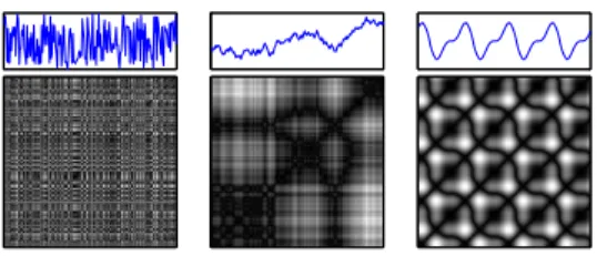
The equation indicates that the recurrence plot consists in a binary image in which dots only indicate if there is a recurrence of a state or not. What sets the value of each point in the image is the closeness threshold. However, determining an appropriate value for this parameter is not intuitive. Addi-tionally, there may exists loss of information when the matrix is binarized. However, we can skip the binarization step and use color information in the image. With this modification, the RP shall represent the distance between the states in the space, instead their recurrences [6]. Fig. 2 shows three examples of unthresholded RPs, in different degrees of randomness.
Fig. 2. Time series with different degrees of randomness (top) and their respectives recurrence plots (bottom): totally random noise (left); random walk (middle); periodic composition of sine and cosine (right)
C. Texture Analysis
Texture is a concept that has undergone many attempts of definition by different researchers. In this paper, we understand an image texture as a function of the spatial variation in pixel intensities (gray values) [7]. In order to characterize and quantify a texture, we need a texture descriptor. In this paper, we use four methods as texture descriptors, described next:
Local Binary Pattern. The LBP is one of the most used texture descriptors in image analysis [8]. This method was introduced by Ojala et al. [9] and uses a grayscale and a LBP operator on a circular neighborhood to describe the local texture of an image. Basically, the intensity of a central pixel gc is compared with P pixels gp at the radius R of a circular neighborhood. In order to guarantee that the values are independent of changes in the grayscale, it is considered only the signs of the results rather than the exact values. In the original version, the LBP operator is defined as
LBPP,R =Pp=0−1s(gp−gc)2p. In this paper we evaluated
some extensions of the original operator that has shown better results: uniform operatorLBPP,Ru2, rotation-invariant operator
LBPP,Rri and rotation-invariant uniform operatorLBPP,Rriu2. We performed our experiments withP = 8and R={1,2,3}. A detailed description of these operators can be found in [10].
Grey Level Co-occurrence Matrix.The GLCM [11] is a statistical way to describe an image using second-order texture measures. The method uses spatial dependence between pixels and creates statistics that consider the direction, distance and relation of pixel pairs. Specifically, it describes the frequency of one gray tone appearing in a specified spatial linear relation-ship with another gray tone. The gray co-occurrence matrices are computed in0◦,45◦,90◦and135◦directions. In this paper, we evaluated 20 different relations:angular second moment, entropy, dissimilarity, contrast, inverse difference, correlation, homogeneity, autocorrelation, cluster shade, cluster promi-nence, maximum probability, sum of squares, sum average, sum variance, sum entropy, difference variance, information measures of correlation, maximal correlation coefficient, in-verse difference normalized, and inverse difference moment normalized. These statistics are computed in all four directions and with distances d ={1,2,3,4,5}. A detailed description of these statistics can be found in [11], [12].
Gabor filters.A gabor filter bank [13] is a pseudo-wavelet filter bank where each filter generates a near-independent estimate of the local frequency content. Gabor filter acts as a local band-pass filter with certain optimal joint localization properties in the spatial domain and spatial frequency domain. To extract the Gabor features of a given input image, the image is convolved by a Gabor Wavelet Transform with a set of Gabor filters of different orientations and spatial frequencies that cover appropriately the spatial frequency domain. The convolution output at each point is the information about the spatial relationship between pixels and their neighborhoods. Texture feature vector is made up of the results from all wavelet transforms [14]. We performed our experiments with 5 wavelets scales and 6 filters orientations.
Segmentation-based Fractal Texture Analysis. The SFTA [15] consists in decomposing the input image into a set of binary images from which the fractal dimensions of the resulting regions borders are computed in order to describe
segmented texture patterns. In the analysis of texture, the fractal dimension, which is a measure of the irregularity degree of an object, describes a certain property of the texture. The fractal model is essentially based on the estimation by spatial methods of the fractal dimension of the surface representing the grey levels of the image. Although it is a recent approach, the authors show that the method outperformed other texture feature descriptors such as GLCM and Gabor filter banks, achieving higher precision and accuracy for image classifica-tion and content-based image retrieval tasks.
III. RELATEDWORK
To the best of our knowledge, there are only two papers in the literature that extract texture features from recurrence plots. However, these studies address specific applications and perform a limited texture analysis from a single method or do not use more sophisticated machine learning classifiers.
For instance, in [16] is presented a method for detecting environmental changes in the reinforcement learning. The proposed method uses recurrence plots of state transitions of the system, and quantifies changes of the recurrence plot by a texture analysis, more specifically using GLCM.
In a particular application of human activity recognition [17], the use of geometric properties of high-dimensional video data and the quantification of this geometric information is proposed in terms of recurrence textures. Basically, the human activities recorded by cameras are represented by recurrence plots and these activities are classified by an 1-NN classifier based on LBP features from these plots.
Even without extracting texture features, the most similar work to ours is presented by Silva et al. [2] with the Recur-rence Patterns Compression Distance (RPCD) for time series classification. The RPCD applies a video compression based distance measure (CK-1) in an 1-NN algorithm to estimate the similarity between two time series represented by recurrence plot. Unlike other methods of the literature that extract explicit features directly related to the image texture, the distance mea-sure applied by RPCD is based on the Kolmogorov complexity to compare the texture similarity between two images. To do this, CK-1 exploits the resultant compression of a synthetic video created from the two images to be compared [3].
IV. PROPOSEDMETHOD
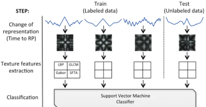
The main idea of the proposed method for time series clas-sification is based on the use of recurrence plot representation and the extraction of texture features of these images. We can see in Fig. 3, an illustrative scheme of our method.
The texture features are used as input attributes for a machine learning algorithm, specifically the Support Vector Machine (SVM) [18]. The choice of SVM is justified by the fact of that this algorithm has demonstrated excellent performance in a variety of pattern recognition problems, such as image classification [19]. In addition, SVM has shown good capability of generalizing in high-dimensional spaces, such as our texture patterns [20].
The texture features were extracted using Local Binary Patterns (LBP), Grey Level Co-occurrence Matrix (GLCM), Gabor filters, and Segmentation-based Fractal Texture Analysis
! & ' $ # # $ ! ! # & ' & '
Fig. 3. Illustrative scheme of our method Texture Features from Recurrence Patterns – TFRP.
(SFTA). We propose the combination of all extracted texture features, since our preliminary results showed that no single approach presented superior performance compared to the others. We also evaluated the accuracy performance of our method with a reduced number of features. Along the text, we use the term Texture Features from Recurrence Patterns – TFRP – to refer to the proposed method1.
V. EXPERIMENTALEVALUATION
We performed our experimental evaluation using a large set of time series classification data from different domains. All data sets can be found at the UCR Time Series Archive [21]. These data sets have standard partitions of training and testing, further facilitating the execution of experiments and the com-parison of results. Similarly to [2], we decided to exclude all synthetic data sets since they were generated for a specific purpose or algorithm. Thus, we use 38 data sets in our experiments. The use of benchmark data sets facilitates the reproduction of our results and the direct comparison with other methods proposed in the literature.
SVM have some parameters that can significantly influence its performance. Therefore, the first step of our experiments consists in a search for the parameters values that maximize the classification accuracy. We varied the parameterscandγ using the Grid Search technique [22], and the choice of kernel (Polynomial and RBF). Given values of minimum, maximum and step size, we evaluated the accuracy of each combination of parameters using a cross-validation approach in training set, since the use of test data is restricted to the final classifier evaluation.
Given the significant amount of features (we have 823 features in total) and the presence of potentially redundant information, we also conducted a feature subset selection step. Thus, we have a reduced number of features that contemplate different views of texture analysis. We employed two well known filter methods for this step: Correlation-based Feature Selection (CFS) [23] and ReliefF [24]. The thresholds used for ReliefF were 5%, 10% and 20% of all 823 attributes.
Our results are reported in Table I. In this table, TFRP20 represents the accuracy achieved with 20% (or 164) of all fea-1In order to facilitate the reproduction of this work, we created a web page in which we made available all detailed numerical results and codes: http://sites.labic.icmc.usp.br/vsouza/ICPR2014/
tures selected by the ReliefF. Among all the feature selection settings, this one showed the best results. TFRP represents the accuracy rates achieved by our method with all features. These results are compared with two state-of-the-art methods: 1-NN with Euclidean distance (ED) and Dynamic Time Warping (DTW). We also compare our method against Recurrence Patterns Compression Distance (RPCD).
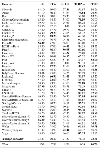
TABLE I. ACCURACY RATES ACHIEVED BY OUR PROPOSED METHOD WITH20%OF ALL FEATURES(TFRP20)ANDTFRPWITH ALL EXTRACTED FEATUES AGAINST1-NNCLASSIFIER USINGEUCLIDEAN DISTANCE(ED), DYNAMICTIMEWARPING(DTW),ANDRECURRENCE
PATTERNSCOMPRESSIONDISTANCE(RPCD).
Data set ED DTW RPCD TFRP20 TFRP
50words 63.10 69.00 77.36 51.87 56.26 Adiac 61.10 60.40 61.64 79.54 79.54
Beef 53.30 50.00 63.33 50.00 63.33
ChlorineConcentration 65.00 64.80 51.09 70.89 70.00 CinC ECG torso 89.70 65.10 97.90 85.22 86.96 Coffee 75.00 82.10 100 96.43 96.43 Cricket X 57.40 77.70 70.77 63.33 64.10 Cricket Y 64.40 79.20 73.85 58.72 63.85 Cricket Z 62.00 79.20 70.77 64.10 63.33 DiatomSizeReduction 93.50 96.70 96.41 92.16 92.48 ECG200 88.00 77.00 86.00 83.00 83.00 ECGFiveDays 88.00 77.00 86.41 84.55 89.55 FaceAll 71.40 80.80 80.95 62.60 71.01 FaceFour 78.40 83.00 94.32 75.00 78.41 FacesUCR 76.90 90.49 94.15 67.22 79.17 Fish 78.30 83.30 87.43 84.57 88.00 Gun Point 91.30 90.70 100 97.33 98.00 Haptics 37.00 37.70 38.64 51.62 46.75 InlineSkate 34.20 38.40 32.00 46.18 48.36 ItalyPowerDemand 95.50 95.00 84.26 93.29 93.78 Lighting2 75.40 86.90 75.41 81.97 85.25 Lighting7 57.50 72.60 64.38 58.90 68.49 MedicalImages 68.40 73.70 71.05 79.08 77.11 MoteStrain 87.90 83.50 79.71 78.59 82.51 OliveOil 86.70 86.70 83.33 90.00 86.67 OSULeaf 51.70 59.10 64.46 89.67 92.98 SonyAIBORobotSurface 69.50 72.50 79.70 87.85 86.86 SonyAIBORobotSurfaceII 85.90 83.10 84.26 88.67 90.77 StarLightCurves 84.90 90.70 88.17 97.91 97.81 SwedishLeaf 78.70 79.00 90.24 92.64 95.04 Symbols 90.00 95.00 90.45 95.78 94.67 TwoLeadECG 74.70 90.40 87.36 98.07 98.86 uWaveGestureLibraryX 73.90 72.70 59.30 58.21 58.74 uWaveGestureLibraryY 66.20 63.40 62.12 59.94 62.31 uWaveGestureLibraryZ 65.00 65.80 61.67 64.91 64.43 Wafer 99.50 98.00 99.66 99.94 99.98 WordsSynonyms 61.80 64.90 72.41 50.47 50.31 Yoga 83.00 83.60 86.60 87.33 85.87 Average accuracy 73.27 76.29 77.57 76.78 78.71 Wins 5/38 7/38 9/38 9/38 10/38
In a general analysis, considering the average accuracy on 38 data sets evaluated, we can see in Table I that both TFRP and TFRP20, outperforms state-of-the-art methods such as 1-NN using ED and DTW. TFRP also slightly outperforms RPCD. In some data sets, we can note a significant difference between our proposed method and the second best method. For instance, we can note a difference of almost 30% between the accuracy of TFRP and RPCD for theOSULeaf data set. For Adiac, the difference is close to 20% and for Haptics, InlineSkate, StarLightCurves, and TwoLeadECG, we outper-formed the second best method with almost 10% of margin.
In terms of number of wins/ties/losses, TFRP also outper-forms all other methods, as can be seen in the last row of Table I. Considering the amount of wins of each method in pairwise comparisons, we can see in Table II that in 38 data sets, the TFRP is the competitor method that have the largest
number of wins against RPCD (22 wins) and TFRP20has the largest number of wins against DTW (21 wins).
TABLE II. AMOUNT OF WINS OF EACH METHOD CONSIDERING PAIRWISE COMPARISONS ON38DATA SETS EVALUATED. IN EACH ROW,
THE BEST RESULT IS IN BOLD. Competitor ED DTW RPCD TFRP20 TFRP Wins against ED — 24 27 22 25 Wins against DTW 13 — 20 21 20 Wins against RPCD 11 18 — 18 22 Wins against TFRP20 16 16 20 — 24 Wins against TFRP 13 18 15 11 —
In order to facilitate the visualization of our results, we also present a graphical representation of the results in Table I. In these plots, each data set is represented by a point where the y coordinate is the accuracy obtained by TFRP and the x coordinate represents accuracy obtained by a competitor method. Thus, points above the main diagonal represent data sets in which TFRP outperformed the competing method. In Fig. 4 we can see ED as competitor method and in Fig. 5 the results against DTW. The number of points above or below the diagonal can be found in Table II.
Fig. 4. Graphical representation of results achieved by TFRP versus 1-NN with Euclidean distance (ED). Each point represents a different data set. The points above the diagonal represent data sets which TFRP outperformed ED.
Fig. 5. Graphical representation of results achieved by TFRP versus 1-NN with Dynamic Time Warping distance (DTW).
The results achieved by TFRP against ED and DTW are very competitive. It is important to note that these methods are considered state-of-the-art in time series classification area and hard to outperform [1]. We can see some points far above the
diagonal, mainly when we consider TFRP against ED. They represent specific data sets where TFRP are far superior to the competing method.
The results against RPCD, the most similar method to ours, can be seen in Fig. 6. The RPCD was recently proposed and showed competitive results against traditional methods.
Fig. 6. Graphical representation of results achieved by TFRP versus Recurrence Pattern Compression Distance (RPCD).
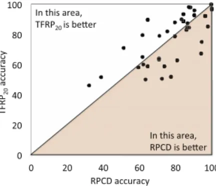
Considering a reduced amount of features of TFRP, we can see in Fig. 7 that TFRP20 presents worse results compared of TFRP, but still shows very competitive results against RPCD.
Fig. 7. Graphical representation of results achieved by TFRP with 20% of all features (TFRP20) versus Recurrence Pattern Compression Distance (RPCD).
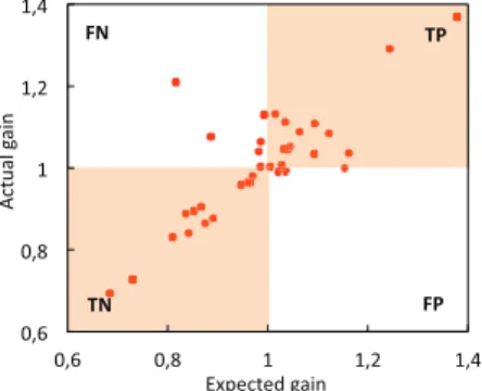
A. The Texas Sharpshooter Fallacy
Many papers in the time series classification literature affirm that their proposed method is useful since it outper-formed the state-of-the-art in some data sets. However, as noted in [25], it is not useful to have an algorithm that can be accurate on some problems unless you can tell in advance on which problems it will be more accurate.
A simple way to show that we can predict when our method will have superior accuracy ahead of time is to use the Texas Sharpshooter plot [25]. To do this plot, we test the accuracy of both TFRP and the competitor method looking only at the training set. We use this information to choose which algorithm will classify the objects from the test set. In order to do that, we can calculate the accuracy gain as:
gain= accuracy(T F RP) accuracy(competitor)
We callexpected gainthe gain calculated over the training set andactual gain the gain over the test set. Recall that the UCR archive provides data sets with standard training and testing splits, and we used these data partitions to calculate the gain values. In order to calculate the gain inside the training set (expected gain) we used leaving-one-out cross-validation, since frequently the training sets have reduced sizes. The Texas Sharpshooter plots are divided in four regions:
• TP.In this region we claimed ahead of time that TFRP would improve accuracy, and we were correct; • TN.In this region we correctly claimed ahead of time
that TFRP would decrease accuracy;
• FN.In this region we claimed ahead of time that TFRP would decrease accuracy, but the accuracy actually in-creased. This represents a lost opportunity to improve, but note that we are no worse off than if we had not tried TFRP;
• FP. This region is the only truly bad case for our method. Data points falling in this region represent cases where we thought we could improve accuracy, but did not.
The plots of TFRP against ED and DTW are presented in Fig. 8 and Fig. 9, respectively. In Fig. 8 we can see only two data sets in the FN region,Hapticsand SonyAIBORobotSur-faceII. This means that for these data sets we could use the TFRP rather than ED for achieve best results. However, we were not able to conclude this from the training set.
"& "' # #$ #% "& "' # #$ #%
Fig. 8. The Texas Sharpshooter plot for TFRP against ED.
In other hand, we can see both in Fig. 8 and Fig. 9 that no data set is located in FP region. This result is very positive for our method, once, based on training data, we never expect that the TFRP achieves better results without it being really true. Thus, we have more confidence in suggesting a particular method for classify an unknown time series data set.
A similar behavior can be seen in Fig. 10 when we comparing TFRP against RPCD. But, in this case, we have a few number of data sets in the FP region. However, these data sets are located very close to border areas that do not represent bad cases. More specifically, we have 30 data sets (78.95%) located in TP and TN regions and 8 data sets (21.05%) located in FN and FP regions.
Fig. 10. The Texas Sharpshooter plot for TFRP against RPCD.
VI. CONCLUSIONS
We presented in this paper a method for time series clas-sification based on texture features extraction from recurrence plots. We evaluated the combination of all extracted features and the use of a reduced amount of features in a SVM algorithm.
In an experimental evaluation performed on 38 data sets, we can note that our proposed method TFRP outperformed the main known competitors in the literature. In many cases, the TFRP20also achieves competitive results even with a reduced amount of features. These results are relevant, as they can be obtained at a lower processing cost.
In future work, we will explore the characteristics of the data sets that showed a high difference between our method and rivals in terms of accuracy. This information can be used in a meta-learning classifier that assists in the choice of the best method according to the data characteristics. This is particularly important when it comes to real applications with unknown data. We will also evaluate the use of ensemble methods in which each classifier is learned over a different feature set, such as a different texture descriptor.
ACKNOWLEDGMENT
This work was funded by CNPq and FAPESP awards #2011/17698-5, #2012/07295-3, #2012/50714-7 and #2013/23037-7.
REFERENCES
[1] H. Ding, G. Trajcevski, P. Scheuermann, X. Wang, and E. Keogh, “Querying and mining of time series data: experimental comparison of representations and distance measures,”VLDB, vol. 1, no. 2, pp. 1542–1552, 2008.
[2] D. F. Silva, V. M. A. Souza, and G. E. A. P. A. Batista, “Time series classification using compression distance of recurrence plots,” inICDM, 2013, pp. 687–696.
[3] B. J. L. Campana and E. J. Keogh, “A compression based distance measure for texture,” inSIAM SDM, 2010, pp. 850–861.
[4] E. Keogh and C. A. Ratanamahatana, “Exact indexing of dynamic time warping,”KAIS, vol. 7, no. 3, pp. 358–386, 2005.
[5] J. P. Eckmann, O. S. Kamphorst, and D. Ruelle, “Recurrence plots of dynamical systems,”Europhysics Letters, vol. 4, no. 9, pp. 973–977, 1987.
[6] J. S. Iwanski and E. Bradley, “Recurrence plots of experimental data: To embed or not to embed?”Chaos: An Interdisciplinary Journal of Nonlinear Science, vol. 8, no. 4, pp. 861–871, 1998.
[7] M. Tuceryan and A. K. Jain, “Texture analysis,”Handbook of pattern recognition and computer vision, vol. 235–276, 1993.
[8] H. R. E. Doost and J. Rahebi, “An efficient method for texture clas-sification with local binary pattern based on wavelet transformation,” IJES, vol. 4, no. 12, pp. 4881–4885, 2012.
[9] T. Ojala, M. Pietik¨ainen, and D. Harwood, “A comparative study of texture measures with classification based on featured distributions,” Pattern Recognition, vol. 29, no. 1, pp. 51–59, 1996.
[10] T. Ojala, M. Pietikainen, and T. Maenpaa, “Multiresolution gray-scale and rotation invariant texture classification with local binary patterns,” IEEE TPAMI, vol. 24, no. 7, pp. 971–987, 2002.
[11] R. M. Haralick, K. Shanmugam, and I. H. Dinstein, “Textural features for image classification,”IEEE TSMC, no. 6, pp. 610–621, 1973. [12] A. Baraldi and F. Parmiggiani, “An investigation of the textural
char-acteristics associated with gray level cooccurrence matrix statistical parameters,”IEEE TGRS, vol. 33, no. 2, pp. 293–304, 1995. [13] B. S. Manjunath and W.-Y. Ma, “Texture features for browsing and
retrieval of image data,”IEEE TPAMI, vol. 18, no. 8, pp. 837–842, 1996.
[14] M. Idrissa and M. Acheroy, “Texture classification using gabor filters,” Pattern Recognition Letters, vol. 23, no. 9, pp. 1095–1102, 2002. [15] A. F. Costa, G. Humpire-Mamani, and A. J. M. Traina, “An efficient
algorithm for fractal analysis of textures,” inSIBGRAPI, 2012, pp. 39– 46.
[16] T. Takahashi and M. Adachi, “A detection method of environmental changes using recurrence plots for reinforcement learning,” inNOLTA, 2005, pp. 246–249.
[17] K. Kulkarni and P. Turaga, “Recurrence textures for human activity recognition from compressive cameras,” inICIP, 2012, pp. 1417–1420. [18] C. Cortes and V. Vapnik, “Support vector machine,”Machine Learning,
vol. 20, no. 3, pp. 273–297, 1995.
[19] S. Li, J. T. Kwok, H. Zhu, and Y. Wang, “Texture classification using the support vector machines,”Pattern Recognition, vol. 36, no. 12, pp. 2883–2893, 2003.
[20] K. I. Kim, K. Jung, S. H. Park, and H. J. Kim, “Support vector machines for texture classification,”IEEE TPAMI, vol. 24, no. 11, pp. 1542–1550, 2002.
[21] E. J. Keogh and S. Kasetty, “On the need for time series data mining benchmarks: a survey and empirical demonstration,” inACM SIGKDD, 2002, pp. 102–111.
[22] C. W. Hsu, C. C. Chang, and C. J. Lin, “A practical guide to sup-port vector classification,” Department of Computer Science, National Taiwan University, Tech. Rep., 2003.
[23] M. A. Hall, “Correlation-based feature selection for machine learning,” Ph.D. dissertation, The University of Waikato, 1999.
[24] I. Kononenko, “Estimating attributes: analysis and extensions of relief,” inECML, 1994, pp. 171–182.
[25] G. E. A. P. A. Batista, E. J. Keogh, O. M. Tataw, and V. M. A. Souza, “Cid: an efficient complexity-invariant distance for time series,”DMKD, pp. 634–669, 2014.