Distortion Correction for Non-Planar
Deformable Projection Displays
through Homography Shaping and
Projected Image Warping
by
Onoise Gerald Kio
A thesis submitted in partial fulfilment for the requirements for the degree of Doctor of Philosophy
at the University of Central Lancashire
i
Declaration
Concurrent registration for two or more academic awards
I declare that while registered as a candidate for the research degree, I have not been a registered candidate or enrolled student for another award of the University or other academic or professional institution.
Material submitted for another award
I declare that no material contained in the thesis has been used in any other submission for an academic award and it is solely my own work.
Collaboration
The work presented in this thesis was carried out at the Applied Digital Signal and Image Processing (ADSIP) Research Centre, University of Central Lancashire. The work described in the thesis is entirely the candidate’s own work.
Signed:
Type of Award: Doctor of Philosophy Department: School of Engineering
ii
Abstract
Video projectors have advanced from being tools for only delivering presentations on flat or planar surfaces to tools for delivering media content in such applications as augmented reality, simulated sports practice and invisible displays. With the use of non-planar surfaces for projection comes geometric and radiometric distortions. This work dwells on correcting geometric distortions occurring when images or video frames are projected onto static and deformable non-planar display surfaces.
The distortion-correction process involves (i) detecting feature points from the camera images and creating a desired shape of the undistorted view through a 2D homography, (ii) transforming the feature points on the camera images to control points on the projected images, (iii) calculating Radial Basis Function (RBF) warping coefficients from the control points, and warping the projected image to obtain an undistorted image of the projection on the projection surface.
Several novel aspects of this work have emerged and include (i) developing a theoretical framework that explains the cause of distortion and provides a general warping pattern to be applied to the projection, (ii) carrying out the distortion-correction process without the use of a measuring calibration image or structured light pattern, (iii) carrying out the distortion-correction process on a projection display that deforms with time with a single uncalibrated projector and uncalibrated camera, and (iv) performing an optimisation of the distortion-correction processes to operate in real-time.
The geometric distortion correction process designed in this work has been tested for both static projection systems in which the components remain fixed in position, and dynamic projection systems in which the positions of components or shape of the display change with time. The results of these tests show that the geometric distortion-correction technique developed in this work improves the observed image geometry by as much as 31% based on normalised correlation measure. The optimisation of the distortion-correction process resulted in a 98% improvement of its speed of operation thereby demonstrating the applicability of the proposed approach to real projection systems with deformable projection displays.
iii
Table of Contents
Declaration……… i
Concurrent registration for two or more academic awards……….. i
Material submitted for another award………. i
Collaboration……… i
Abstract……… ii
Table of Contents……….. iii
List of Figures and tables……….. viii
Acknowledgement………. xviii
Abbreviations……… xix
CHAPTER ONE: Project Overview………. 1
1.1 Aims and Objectives……….. 1
1.2 Methodology……….. 5
1.3 Novelty of the Distortion-correction Approach………. 7
1.4 Organisation of Thesis………. 9
CHAPTER TWO: Literature Review………... 11
2.1 Introduction……… 11
2.2 Image Geometric Distortion: Causes and Correction ……….. 11
2.3 Projector-Camera Systems……….. 14
2.3.1 Projector-Camera System Calibration……… 14
2.3.2 Correction of Geometric Distortion for Projected Displays………... 15
2.3.3 Correction of Geometric Distortion for Projected Displays Developed in this Work………. 21
2.4 Image Warping Techniques.………. 23
2.5 Image Similarity Measurement……….. 26
iv
CHAPTER THREE: Theory of Image Processing Techniques………. 29
3.1 Introduction……… 29
3.2 Image Feature Detection Techniques……….. 29
3.2.1 Image Edge Detection……… 30
3.2.2 Image Corner Detection……….. 36
3.2.3 Blob Detection……….. 38
3.3 Projections on Planar Surfaces………. 40
3.3.1 2D Homography……… 40
3.3.2 2D Projection onto the 2D Sensor Plane of a Camera……….. 42
3.3.3 2D Transformations between a Projector, a Planar Projection Surface and a Camera……….. 43
3.4 Straight Line Geometry……….. 45
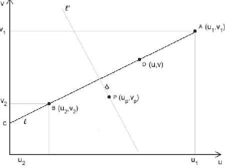
3.4.1 The Equation of a Straight 2D Line……… 46
3.4.2 Estimating the Distortion of a Straight 2D Line……… 47
3.5 Image Warping Techniques………. 48
3.5.1 Translation………. 48
3.5.2 Procustes Transformation……….. 49
3.5.3 Affine Transformation……….. 49
3.5.4 Perspective Transformation………... 50
3.6 Image Warping with Radial Basis Function Interpolation……… 51
3.7 Image Similarity Measurement………. 53
3.7.1 Normalised Cross-correlation Coefficient (NCC)………. 53
3.7.2 Phase Correlation………. 54
3.8 Chapter Summary……….. 55
CHAPTER FOUR: Geometric Distortion Correction for Static Projection Displays 56 4.1 Introduction………. 56
4.2 Illustrating Geometric Distortion of a Straight Line Projected Onto Non-planar Surface……….. 57
v
4.2.2 Algebraic Representation of a Plane and a Cylinder……… 58 4.3 Geometric Distortion Measurement of Image Lines
and Geometric Distortion Correction using a Calibration Image……… 62 4.3.1 The Calibration Image and Measure of Distortion of its
Grid Lines………. 62 4.3.2 Measure of Distortion/Straightness of Straight Lines
in an Image……… 65 4.3.3 Measuring the Distortion of Projected Horizontal and Vertical Lines of the Calibration Image……….. 67 4.3.4 The Geometric Distortion-correction Process………... 70 4.3.5 Experimental Considerations……….... 74 4.4 Results of Distortion-correction Tests with the Calibration Image…………. 75 4.4.1 General Distortion-correction Results………. 75 4.4.2 Results of Tests to Determine the Number of Feature Points
to Use in the Calibration Image……….. 83 4.4.3 Results of Tests to Determine the Type of RBF to Use for
Distortion Correction………. 87 4.4.4 Results of Distortion-correction Tests for Other Non-planar
Surfaces, eg Two Planar Surfaces Meeting at Right Angles……… 88 4.5 Automatic Geometric Distortion-correction Without Using a Calibration
Image……… 92 4.5.1 Edges and Corners at the Periphery of the Projected and
Captured Images used as Feature Points for Distortion Correction. 93 4.5.2 Blobs in the Projected and Captured Images Used as Feature Points for Distortion Correction……… 94 4.5.3 Linear Modelling of Distortion……… 95 4.6 Results of Tests of Automatic Geometric Distortion-correction
Without Using a Calibration Image……….. 98 4.6.1 Edges and Corners at the Periphery of the Projected and
vi
4.6.2 Distortion-correction using Blob Features………... 100
4.6.3 Linear Modelling of Distortion……….. 103
4.7 Chapter Summary……….. 109
CHAPTER FIVE: Geometric Distortion Correction for Deformable and Dynamic Projection Systems……….. 112
5.1 Introduction……… 112
5.2 Illustrating Geometric Distortion of a Warped Image Line Projected onto a Deformable or Dynamic Quadric Surface……….. 113
5.3 Distortion Correction for Real Dynamic Projection Systems……….. 114
5.4 Results of Tests Carried out for Distortion-correction Techniques on Real Dynamic Projection Systems………. 116
5.5 Code Profiling and Optimisation towards Real-time Operation……….. 123
5.5.1 Creating a Region-of-Importance (ROI) for Edge and Corner Detection……… 125
5.5.2 Estimating Corners from Edge Information……….. 128
5.5.3 Using linear Interpolation to Approximate the Warping of the Projected Image……….. 130
5.5.4 Greyscale versus RGB Processing……….. 131
5.5.5 Parallel Processing……… 131
5.6 Results of Code Profiling and Optimisation for Real-time Performance.. 132
5.6.1 Code Profiling Results Obtained from Creating an ROI for Edge Detection and 4 ROIs for Corner Detection……….… 132
5.6.2 Code Profiling Results Obtained from Estimating Four Corners from Detected Edges..………. 133
5.6.3 Code Profiling Results Obtained from Using Linear Interpolation to Approximate the Warping of the Projected Image……….. 136
5.7 Golf Simulation………. 140
5.8 Results from Golf Simulation………. 141
vii
CHAPTER SIX: Conclusion and Recommendations………..……… 146
6.1 Conclusion……….. 146
6.2 Original Contributions………. 148
6.3 Practical Considerations……… 149
6.3.1 Practical Applications……… 149
6.3.2 Image Processing Considerations….……… 150
6.4 Recommendations………. 151
APPENDIX……….. 153
A1 Detection and Arranging Detected Corner Points of the Distorted Projected Calibration Image……….. 153
A2 Obtaining feature points along a distorted edge……….. 157
A3 Graphical User Interface (GUI)……….. 159
viii
List of Figures and Tables
Figure 1: The components of a projector-camera system consisting of multiple projectors, two cameras, a computer and projectionsurface/display………. 2
Figure 2: Block diagram of a projector-camera system showing its components and their functions……….. 3
Figure 3: Optical ‘see-through’ camouflage system applied to the backseat
of a vehicle……… 4
Figure 4: An aboutGolf ltd golf simulator showing its projector, loose screen, and tee area……….. 5
Figure 5: Components of a geometric distortion-correction system and process 7
Figure 6: Generalised block diagram describing the distortion-correction
process for projected displays……… 17
Figure 7: Various projection surfaces used to test distortion-correction
techniques mentioned in literature………. 23
Figure 8: Rapid change of univariate function indicates an edge……….. 31
Figure 9: Laplacian Convolution Kernels………. 33
Figure 10: Comparison of various edge detectors to test their suitability
for detecting projected image features……….. 35
ix
Figure 12: Comparison of the Harris and Stephens corner detector with Shi and Thomasi minimum eigenvalue corner detector in terms
of detected corners and algorithm speed……….. 38
Figure 13: Detecting common blob features between a projected image and the camera image of the projection………. 40
Figure 14: The projection of points from a plane surface to respective points in two image planes……….. 41
Figure 15: Image 𝐼𝑝 projected from the Projector Plane 𝑃 to form an image 𝐼𝑠on the projection surface………. 44
Figure 16: A straight 2D line 𝑙 described by the equation 𝑣 = 𝑚𝑢 + 𝑐………. 46
Figure 17: Translation of a region of pixels in an image……… 48
Figure 18: Procustes transformation of an image………. 49
Figure 19: Affine transformation of an image………. 50
Figure 20: Projective-transformed image with……….. 50
Figure 21: A projection system consisting of a projector, camera, projection surface and computer……….... 57
Figure 22: Geometric illustration of the projection of a 2D image line onto a 3D or non-planar surface……….. 59
x
Figure 23: Plots of the profile curve of a horizontal line projected
onto a quadric (cylindrical) surface……… 61-62
Figure 24: Calibration image consisting of 14×14 feature points projected
onto the non-planar surface to measure and correct projected image distortion 64
Figure 25: Camera capture of the calibration image projected onto the non-planar projection surface showing the detected corner points, horizontal and vertical lines formed by linking two extreme corner points, and the quadrilateral formed by linking the corner points at the four corners of the image……… 64
Figure 26: A plot of average deviation of member feature points from
the horizontal and vertical lines shown in figure 25………... 65
Figure 27: 200 Randomly-generated image lines………. 66
Figure 28: Plot of average deviations for lines shown in figure 27……….. 67
Figure 29: Histogram showing the distribution of average deviation values
for the 200 randomly-generated lines in figure 27……….. 67
Figure 30: Histograms of distributions of average deviations of points from the projected vertical lines of the calibration image and average deviations of points from 200 randomly-generated straight
xi
Figure 31: Histograms of distributions of average deviations of points from the projected horizontal lines of the calibration image and average deviations of points from 200 randomly-generated straight
image lines………. 69
Figure 32: Histograms of distributions of average deviations of points
from the projected horizontal lines and vertical lines of the calibration image and average deviations of points from 200 randomly-generated straight
image lines……… 69
Figure 33: Illustration of the respective positions of the distortion-corrected line 𝑙, a line 𝑙′ perpendicular to it, and distorted feature point 𝑝𝑑 opposite
point 𝑝𝑑′ and distortion-corrected point 𝑝𝑟……….... 71
Figure 34: Image of a calibration image showing correctly detected
feature points, missing and unwanted feature points………. 74
Figure 35: Geometric distortion correction of the projection of a
calibration image consisting of 196 feature points……….. 76-77
Figure 36: Geometric distortion correction of the projection of a natural image replacing the calibration image and using the warping coefficients
obtained from the calibration image………. 78-79
Figure 37: Average deviation of feature points from their respective horizontal and vertical lines on the observed images of projection of the
calibration image………. 80
Figure 38: Normalised Correlation Coefficients (NCC) of the observed
xii
Figure 39: Peak NCC values for distorted and distortion-corrected projections using 100, 144 and 196 feature points………. 82-83
Figure 40: Results to demonstrate the need for having a sufficiently high number of feature points for the calibration image to achieve better
geometric distortion correction………. 84-85
Figure 41: Curve sections with varying number of feature points
to be used as RBF control points to warp the curve sections into the straight
horizontal lines……….. 86
Figure 42: Comparison of three RBF types based on the NCC values of
distortion-corrected images……… 87
Figure 43: Distortion-Correction Results for 2 planar surfaces meeting at
right angles………. 89-92
Figure 44: Illustration of a warped projected image showing the initial edges, the final edges after warping and the initial and final points along each edge. 96
Figure 45: Illustration of the assumed linear relationships between
coordinates of points in the unwarped and warped images………... 97
Figure 46: Results of auto geometric distortion correction
by RBF warping using 28 control points from the top and bottom edges
of the projected image………. 98-100
Figure 47: Results of auto geometric distortion correction by RBF warping
xiii
Figure 48: Box and whisker plots for a single image showing the absolute difference between horizontal and vertical pixel coordinates obtained from using a calibration image and coordinates obtained from linear
interpolation of coordinate displacements………. 105
Figure 49: Comparison between pre-warped projected images by
RBF coefficients obtained from using a calibration image and RBF coefficients obtained from linear interpolation of deviation of control points on the
periphery of the projected image………. 105-106
Figure 50: Observed geometrically distorted projection and
distortion-corrected projections for methods involving the use of the 196-point calibration image and that obtained from using 52 known control point displacements and 144 linear interpolated control
point displacements……… 107-108
Figure 51: Improvement of peak NCC matching values between the desired observed projection and the observed distorted projection and distortion-correction by linear interpolation of control point displacement for 10 different poses of the projector, camera and shapes of the
projection surface……… 108
Figure 52: Curves showing the profiles of the warped and unwarped projected lines and their respective profiles on the quadric projection
surface before and after the change of shape of the projection surface 113-114
xiv
Figure 54: Results for successively correcting, distorting,
and correcting the observed projection by warping the projected image
from its previously-warped state……… 117-119
Figure 55: Graph showing peak NCC values for successively correcting, distorting, and correcting the observed projection by warping the
projected image from its previously-warped state………... 120
Figure 56: Results for successively correcting, distorting, and correcting the observed projection by warping the projected image from
its unwarped state……… 120-122
Figure 57: Graph of peak NCC values obtained from successively correcting, distorting, and correcting the observed projection by warping the
projected image from its unwarped state……… 123
Figure 58: Illustrating the principle of developing ROIs for faster edge
and corner detection……….. 125
Figure 59: Observed consecutive frames of a projection on a surface hit by a projectile in an experiment to investigate the deviation of feature points from one frame to the next on a deforming projection surface………….. 126
Figure 60: Observed displacement of edge pixels in the horizontal and
vertical image directions after striking projection surface with a projectile 127
Figure 61: Two-dimensional variation of the four corners of observed
projected video frames on a deforming surface………. 128
xv
Figure 63: Pictorial illustrations to show the closeness between estimated corners and actual corners……… 134
Figure 64: Comparison between values of estimated and true corner points using cosines of angles and absolute magnitude differences
between their respective vectors………. 135
Figure 65: Comparison between 3 methods used to warp the 640 x 480
pixel sized projected image……….. 137-138
Figure 66: Geometric distortion correction process for simulated golf 140
Figure 67: Projected image of a golf course and distortion-corrected
frames of the projection after projectile hits the projection surface…. 141-143
Figure 68: Peak NCC values for distorted and distortion-corrected frames
of the golf-simulation test……… 144
Figure 69: A chosen corner point and its four closest neighbours…….. 154
Figure 70: Flow diagram of steps used in producing an ordered set of
corner points from an unordered set of points………. 156
Figure 71: Camera view of the calibration image showing misarranged
and correctly-arranged corners………. 156-157
Figure 72: Edge image of the projection showing red non-distorted
xvi
Figure 73: A typical top peripheral section of the camera image of the projection showing the distorted edge with the a distorted feature point, the desired non-distorted edge with a non-distorted feature point,
the perpendicular line, and other detected feature points in the image…… 158
Figure 74: GUI created in Matlab……….. 160
Table 1: Convolution kernels for gradient-based edge detectors……… 32
Table 2: Examples of Radial basis functions……… 53
Table 3: Comparing approximate minimum and maximum deviations in 2 image directions for horizontal and vertical lines of the projected
calibration image……… 65
Table 4: Comparison of three RBF types based on the average computation time to warp a 640×480 pixel image……… 88
Table 5: Average time taken for critical image distortion-correction
operations to complete on Matlab……….. 124
Table 6: Comparison between estimated mean coordinates of corners obtained from the first frame of a video and their actual mean coordinates obtained from the whole video duration……… 130
Table 7: Processing time saving resulting from creating ROIs for edge
and corner detection………. 132
Table 8: Processing time saving resulting from creating 2 ROIs for
xvii
Table 9: Processing time saving resulting from using linear interpolation to warp most of the projected image of size 640 x 480 pixels rather than
evaluating the warping function to warp the whole image………. 136
Table 10: Summary table showing all image processing time savings
xviii
Acknowledgement
I wish to thank God for giving me the strength, patience and enablement to carry out this work.
Special thanks to my darling wife Jumoke and daughter Annabelle, my mother Agatha, and members of my extended family for their support and encouragement.
My profound gratitude goes to the Niger Delta Development Commission of the Federal Government of Nigeria (NDDC) that sponsored my studies at the University of Central Lancashire, United Kingdom.
I wish to acknowledge the invaluable guidance of members of my supervisory team including my Director of Studies Professor Lik-Kwan Shark, and my co-supervisors
xix
Abbreviations
ASIFT: Affine Scale-Invariant Feature TransformCFD: Computational Fluid Dynamics CMM: Coordinate Measuring Machine CSS: Curvature Scale Space
CT: Computed Tomography DIA: Document Image Analysis DoG: Difference of Gaussians DirectAR: Direct Augmented Reality
FAST: Features From Accelerated Segment Test GPU: Graphics Processing Unit
GUI: Graphical User Interface GSIFT: Geometric SIFT
HWD: Head Worn Display LoG: Laplacian of Gaussian
NCC: Normalised Cross Correlation OS: Operating System
PCA-SIFT: Principal Components Analysis – Scale Invariant Features Transform RBF: Radial Basis Function
ROI: Region of Importance/Interest SIFT: Scale-Invariant Feature Transform SURF: Speeded-Up Robust Features
SUSAN: Smallest Univalue Segment Assimilation Nucleus SVD: Singular Value Decomposition
2D: Two Dimension(al) 3D: Three dimension(al)
1
CHAPTER ONE
Project Overview
1.1 Aims and Objectives
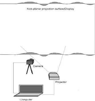
The aim of this work is to correct geometric distortion observed when undistorted images and video frames are projected onto both static and dynamic/deformable non-planar projection surfaces or displays. The work features a projection system consisting of a projector projecting images and video from a computer onto the projection surface, a single uncalibrated camera that monitors the projections on the surface, and the computer providing image processing and system control.
Homography Shaping is a term used in this work to describe the derivation of the shape of the distortion-corrected projection. Through homography shaping, the desired observed projection is made to look like the projection was done on a planar surface. The homographies or 2D transformations between the image being projected, the desired image on the projection surface, and the camera image of the projection are defined in Section 3.3 and the distortion correction process through homography shaping is explained in Section 4.3.
Image Warping is generally a transformation that changes the spatial configuration of an image [1]. In this work image warping is the process of transforming the spatial configuration of the image being projected in order to observe its non-distorted projection on the non-planar projection surface. The term pre-warping is also used in this work to refer to the warping of the image being projected for the same purpose. The simple-to-apply Radial Basis Function (RBF) interpolation is used to implement the warping of images.
2
(i) The distortion-correction system developed will work automatically without needing a calibration image or structured light pattern to first estimate or measure the level of distortion on observed projections brought about by the non-planar surface.
(ii) The distortion-correction system will be able to operate in real-time in order to be used to correct distortions in practical projection systems including optical camouflage systems deployed in vehicles and computer-simulated golf systems, both described in the following paragraphs.
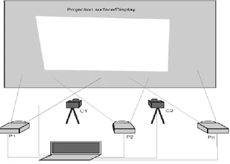
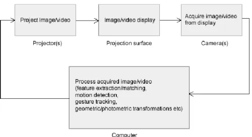
The arrangement of a projection system using cameras for feedback and computer for processing and control is shown in figure 1 while the block diagram describing the system functionality is shown in figure 2.
Figure 1: The components of a projector-camera system consisting of multiple projectors (P1, P2 ... Pn), two cameras (C1, C2), a computer and projection surface/display.
3
Figure 2: Block diagram of a projector-camera system showing its components and their functions.
Conventional standalone projectors are used to provide visual content from computers onto planar or slightly curved surfaces to audiences. These projection systems do not introduce noticeable geometric distortion to the observed visual content as straight projected lines and curves are viewed respectively as straight lines and curves with perspective transformation brought about by the relative position of the projector, projection surface and viewpoint of the observers.
Apart from delivering presentations to audiences, projectors have been used in a variety of ways to either enhance the functionality of some existing systems or form integral parts for others. For example in a prototype system described in [2] a projector is used to deliver structured light pattern to a laparoscope (a surgical device for viewing internal structures of the body) to aid in the acquisition of 3D video data of a surgery site. Through an enhanced Head Mounted Display the user can perform operations having 3D video data from both the enhanced laparoscope and an augmented video source. Projectors are used to project images onto real objects to enhance their appearance and make them more compelling to viewers. In such systems [3] video cameras are used to acquire projected images and images of the environment for system calibration and measurement of the environment in order to provide seamless registration of images on the target objects from multiple projectors. Similarly, the authors in [4] describe a projection system that changes the appearance of objects by making them look like other objects. With the images of the target object
4
acquired by the camera, a compensation image is derived from photometric properties of the object, its environment, and that of the camera and projector.
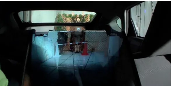
An optical camouflage system [5] allows users ‘see through’ opaque objects like the rear seat of a vehicle. For its vehicular application, the system consists of video cameras mounted at the back of the car, a projector mounted behind the front seats, and a rear-facing half mirror mounted above the projector. The projector projects the portion of the view of the outside of the car provided by the camera but not visible to the driver onto the half mirror which reflects the projection onto the back seat. This results in a complete view of the rear of the car.
Figure 3: Optical ‘see-through’ camouflage system applied to the backseat of a vehicle.
Computer-based golf simulators enable golfers to practice golf indoors. They consist of a loose screen attached to a housing onto which the image of a fairway or part of a golf course is displayed by a projector, arrays of sensors (usually infrared) to sense the movement of the ball from the tee to the screen after being struck by the player, and a computer which collects and processes the ball-tracking signals and performs other image processing and control functions for the system [6]. The projector also projects the computer-generated video of the flight of the ball through the section of golf course. The illustration of a golf simulator is given in figure 4.
5
Figure 4: An aboutGolf ltd golf simulator showing its projector, loose screen, and tee area [7]
Projecting images and video on non-conventional (for example non-planar, coloured and/or textured) projection surfaces may introduce undesirable forms of distortion. Geometric distortion whereby shapes of projected images become altered to the observer would occur on the non-planar backseat of a car having the optical camouflage system (figure 3) and on the non-planar simulated golf screen as it is struck by the golf ball. Radiometric distortion whereby projected colours change as a result of the mixing of colours between the projection and the projection surface would also occur in both systems. Both forms of distortion need correcting for better user satisfaction and many researchers have developed various approaches to mitigating them. A discussion of the most relevant distortion-correction approaches is presented in the literature review of Chapter 2.
1.2 Methodology
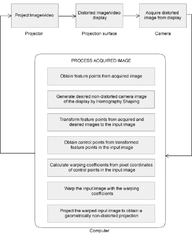
The block diagram describing the connection of components and highpoints of the processing done by the computer in correcting geometric distortion for projected displays is given in figure 5. An elaborate description of the whole process is given in Section 4.3. The process starts by projecting an image or video from the memory of the computer onto the non-planar surface and obtaining a snapshot of the projection with the camera. This snapshot represents the image seen by the observer. Next, feature points including edges and corners of the image obtained by the camera are detected. The detected feature points
6
are then used to measure the amount of geometric distortion in the image. A significant amount of distortion informs the choice of the decision of the system to carry out the distortion correction and the appropriate image warping direction. Next, the feature points are used to construct the desired non-distorted image (the standard) and obtain a 2D homography between the camera image and the projected image (the input image). Transformation of the same feature points from the camera image to the projected image yield control points. These control points are used to calculate the RBF coefficients needed to warp them in the predetermined image warping direction. The RBF coefficients so obtained are then used to warp all the pixels of the projected image. The system then re-projects this warped image to give a non-distorted view of the projection. An image of the distortion-corrected projection may be obtained by the camera and compared with the standard to measure the effectiveness of the correction process.
7
Figure 5: Components of a geometric distortion-correction system and process
1.3 Novelty of the Distortion-correction Approach
This work has a number of novelties when compared with some other distortion-correction systems discussed in Section 2.3. The individual novelties are presented in Chapters 4 and 5 and include:
8
(i) This work presents a geometric and algebraic explanation on how geometric distortion occurs when projecting an image from a plane to a non-planar surface in Section 4.2. The derivation of the direction of warping of the projected image is also given. This treatment of the distortion generation and correction process for projected displays can be developed further into a standard distortion-correction simulation tool for future applications.
(ii) The distortion-correction process for a dynamic system with a deformable projection surface whose shape changes with time presented in this work is monocular, does not require the calibration of neither the projector nor the camera, and does not require the 3D measurement or construction of the projection surface. It is therefore a less costly alternative in terms of system components and processing requirements than the calibrated binocular dynamic distortion-correction system described in Section 2.3.
(iii) By taking advantage of the nature of the projection surface, important assumptions on the distortion pattern of the non-planar projection surface are made in Section 4.5.3 of this work. The resulting distortion-correction system developed does not therefore require the projection and detection of any structured light pattern or calibration image on the projection surface as some other systems like [8] do. The need for developing imperceptible patterns and detection algorithms for them is also avoided. Imperceptible patterns are very difficult to extract because of the radiometric modulations that the projection surface and noise add to the camera-captured image. The distortion-correction system developed in this work can therefore be used in static and dynamic projection systems without any interruptions.
(iv) A much simpler RBF interpolation approach to warping as opposed to other processing-demanding warping methods like Bezier patches used in other systems is presented in this work. The optimisation of the RBF image warping algorithm yielding a time saving of 99.32% (Section 5.6) for real-time operation is also presented in this work. Practical applications include possible presentations in places where there is no planar projection surface. For viewers to enjoy a distortion-free view they should have similar field of view as the camera used to observe the surface because the distortion correction is carried out through the
9
viewpoint of the observing camera. A method by which distortion correction may be achieved for more than one view is given in Chapter 6. In simulated golf practice the user plays the golf ball against a deformable surface that dampens the motion of the golf ball and prevents injury to the player as the ball rebounds off the surface. The trajectory of the golf ball and some text telling its measured speed may also be displayed on the surface. The player’s experience will also be improved by removing the geometric distortion from the entire projection as the ball strikes the projection surface.
1.4 Organisation of Thesis
Chapter 2 is a combined review of already-developed techniques for solving image distortion problems in some areas of computer vision including projector-camera systems. It also includes popular image warping techniques.
Chapter 3 presents the theories behind all the projective transformations and image processing techniques used in this work. It discusses the 2D image homography transformations, popular techniques for detection of feature points in images, various methods of warping an image with illustrations, important concepts of straight-line geometry and its application in measuring geometric distortion in an image, and various methods used in matching or comparing images that give an indication of how much the geometries of a set of images differ from each other.
Chapter 4 presents the techniques developed in this work to correct geometric distortion for static projection displays. It begins by explaining the cause of distortion when a straight line is projected onto a non-planar surface and develops a framework on how this sort of distortion can be solved by warping or changing the shape of the original projected line. It also presents a method to evaluate the distortion/straightness of ‘straightest’ lines in an image in order to create a basis to compare the distortion values of detected lines in real images.
10
It combines the warping framework developed earlier with image feature point detection methods, 2D image transformations and the RBF image warping method presented in Section 3.6 to solving geometrical distortion problems in actual projected displays.
Geometric distortion-correction techniques presented in Chapter 4 include one that relies on a calibration image and others that do not require its use. The results of various tests performed with the projector-camera distortion-correction system are also presented.
Chapter 5 extends techniques developed in Chapter 4 to correcting geometric distortion problems in deformable projected displays. It discusses ways by which image processing algorithms used for the correction process can be optimised for real-time operation. It also presents various tests and results to validate these techniques including their application to simulated golf, where the golf system is simulated by striking the projection surface with a projectile.
A general discussion of the whole work including techniques developed and the results obtained is given in Chapter 6. Recommendations for improvement of this work concludes the chapter. Image processing methods not elaborately mentioned in the main body of this thesis are presented in an appendix.
11
CHAPTER TWO
Literature Review
2.1 Introduction
In this chapter a survey is carried out to identify the important aspects of this work: (i) the prevailing problem of geometric distortion in images acquired by a typical computer vision system and (ii) the techniques developed to correct it. In Section 2.2 the concept of geometric distortion in images is defined and a survey on its causes and methods developed by researchers to correct it is presented. The focus of this work is correcting geometrically- distorted projections from images of the projection acquired by a camera. Section 2.3 therefore gives a survey of similar projector-camera systems. The survey discusses the projector-camera system calibration and various techniques developed to correct similar geometric distortion problems. Techniques developed to correct geometric distortion on projected displays involve a number of parametric and non-parametric geometrical image transformation or warping techniques. A brief description of these warping techniques is given in Section 2.4. A more detailed description of specific image processing techniques with their underlying mathematical expressions is given in Chapter 3. Image processing techniques used to measure the similarity between images are presented in Section 2.5. A summary of the main discussions in this chapter is presented in Section 2.6.
2.2 Image Geometric Distortion: Causes and Correction
Geometric distortion in an image occurs when the geometry of objects in the image differ from the geometry of respective objects in the scene, in ways that the intended purposes of the vision system, such as measurements or object recognition tasks may not be able to be performed because of the distortion. Geometric distortion may present itself as straight lines from the source scene appearing as curves in the image caused by the lens of the camera, the change in perspective such that relative dimensions of objects in the image are not represented as they are in real life because their respective shapes become skewed, objects in the image appearing blurred due to the motion of the camera or the objects in
12
the scene, or the occlusion of important objects in the image by unwanted objects in the scene may occur.
Geometric distortion occurs in various fields that utilise imaging systems to acquire and analyse images and it may be caused by any of three elements of imaging systems: (i) the nature of the scene or image source, (ii) the medium through which light rays travel to get to the image acquisition device, and (iii) properties of the target acquisition device (a camera for example). The following paragraphs describe various forms of geometric image distortions caused by the various elements of imaging systems and techniques developed to correct them.
The source of the imaging system is the scene object being photographed or studied. Various image sources are encountered in computer vision. In [9] geometric distortion is caused by the non-planar or rumpled paper documents from which images are acquired. To solve the distortion problem, the 3D shape model of a document is constructed from a smooth shading image acquired by Digital In-painting and a 2-pass Shape-From-Shading technique, then flattened to restore the shape of the document to its assumed pleasant planar view. As stated in [9], this type of geometric correction can be used as a preliminary restoration step in Document Image Analysis (DIA) systems. Several other methods to correct the geometric distortion of images of documents caused by the non-planar shape of the source objects have also been developed in [10], [11], and [12]. In [10] for instance, the surfaces of the documents whose images were rectified were modelled as cylindrical surfaces. The geometrical rectification of the images was achieved by estimating the extent of bending of the document surfaces using the mapping of points from the scene to points in the image and using this information to digitally lay the image out to make it appear flat.
A typical area where the transmission medium causes geometric distortion of acquired images is underwater imaging. Distortion of the image of an object in water may be caused by the rapid flow of water in the scene, image noise caused by floating particles, or motion blur or refraction of light waves at the water-air interface.
13
In [13] it is assumed that geometric image distortion is only caused by dynamic refraction at the water surface and presents itself as motion blur in the acquired images. The dynamic refraction was caused by both unidirectional cyclic waves and circular ripples. The distortion-correction or ‘deskewing’ process therefore involved correcting distortions caused by both kinds of water waves. While carrying out 3D measurements of objects in water using a fish-eye stereo camera, [14] used a ray-tracing method involving modelling the refraction of light from air to the water surface by Snell’s law to account for the geometric distortions present in the stereo images. On the other hand, by utilising the distortion phenomenon caused by the refraction of light rays through an air-water medium differently, a method of reconstructing the surfaces of transparent non-rigid bodies like water by measuring the geometric distortion of objects lying underneath them was developed in [15]. This method first models the apparent movement of the object underneath the transparent surface using optical flow, extracts the optical flow parameters and then reconstructs the surface using the estimated surface normals.
Geometric distortions in images introduced by the target camera can either be caused by the camera lens or sensor. Lens distortion is caused by the spherical shape of the camera lens and it manifests as straight lines in the scene appearing as curved lines in the image. Lens distortion can be grouped into 3 types according to [16]: (i) shift of optical centre which occurs when the camera sensor is shifted in the optical plane, (ii) radial distortion which includes barrel distortion when straight lines appear curved and bend away from the centre of the image or pincushion distortion when straight lines appear curved and bend towards the centre of the image, and (iii) decentering distortion, which occurs when the fixation of the lens is not orthogonal with respect to the image sensor and optical axis thereby causing image distortion in a direction that is tangential to radial distortion. The more prevalent radial lens distortion has been modelled in various ways in reducing its effects in imaging systems and it is essentially part of the camera calibration process. Examples are seen in [17], where distortion in the two image directions is approximated to a 2nd degree polynomial in 𝑟 the radius of distortion, and [18] where higher-degree polynomials are obtained and solved through a covariance line-rectification method.
14
2.3 Projector-Camera Systems
Cameras are incorporated into the computer-projector loop (figures 1 and 2) to monitor the display of a projector. Such systems may also be called smart projection systems because of the automatic problem-solving functions they perform. A projector-camera system consists of one or more projectors, one or more cameras, and one display surface either planar or curved, plain or patterned, or consisting of a combination of a number of surfaces. The purpose of the camera is to monitor what is being projected onto the display surface by the projector by capturing projected images. Further processing can be done on the captured images by appropriate software running on a computer. This processing may involve projector-camera system calibration, radiometric and geometric distortion correction of the projected images, shadow elimination from the display surface [19], or creating a seamless arrangement on the display surface of multiple images from multiple projectors.
2.3.1 Projector-Camera System Calibration
Projector-camera system calibration involves estimating the intrinsic and extrinsic parameters of the projector and camera or deriving their respective calibration matrices. Projectors and cameras are usually modelled with the same calibration parameters as the pinhole camera. Various methods of calibrating a projector-camera system exist depending on what is to be achieved in each application. Examples are seen in [20] and [21] where the projector-camera system is calibrated for 3D measurements and modelling respectively. The two-step calibration method described in [20] estimates the intrinsic and extrinsic parameters of the camera and projector. A structured light pattern or calibration image consisting of a grid of black squares on a white background is pasted on the bottom half of a planar projection surface. The 3D coordinates of the corners of the square with respect to the coordinate frame of the projection surface are known. The projector is used to project a calibration image consisting of the same gridded pattern on the top half of the projection surface. Several images of the patterns on the top and bottom halves of the projection surface are captured by the camera at different poses. Correspondences between the coordinates of the feature points of the pasted pattern on the bottom half of
15
the projection surface and the feature points on the camera images are used to estimate 2D homographies between the camera planes and the projection surface. These homographies are then used to estimate the intrinsic and pose parameters of the camera. The 3D coordinates of the feature points of the projected pattern on the top half of the projection surface are estimated by back-projecting the 2D feature point coordinates obtained from the camera images using the camera calibration parameters so obtained. The correspondences between the coordinates of the feature points on the projected image and the back projected ones are used to estimate 2D homographies between the projector planes and the projection surface. Finally these homographies are used to estimate the intrinsic and extrinsic parameters of the projector.
The calibration method described in [21] first uses the coordinates of corner points in camera images of a checkerboard pattern pasted on the projection surface to estimate the calibration parameters of the camera. It then uses the coordinates of corner points in images of a ray code pattern projected onto the checkerboard pattern to obtain the parameters of the projector. This calibration method also estimates radial lens distortion parameters for both the camera and projector.
A radiometric calibration of a projector can also be carried out to compensate for colour differences between the image being projected and what is observed on the display surface. An example of this kind of calibration is seen in [22] where the fast colour compensation is achieved by colour filters attached to the projector.
2.3.2 Correction of Geometric Distortion for Projected Displays
When projectors are used on flat or planar surfaces and the plane of projection is not at right angles with the principal axis of the display surface, rectangular shapes lose their squareness and appear distorted. Straight lines however remain straight. This type of distortion known as keystone distortion [23] is caused by the pose of the projector with respect to that of the projection surface. Several methods have been developed to automatically correct keystone distortion and two of them are reported in [23] and [24].
16
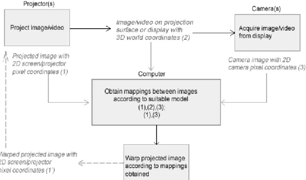
With such applications as virtual and augmented reality or the Office of the Future and Transportation of the Future, it has become imperative to have projectors display content on surfaces that are non-planar or undulating. This kind of projection display however comes with a problem: the surface topography causes a shift in the direction of incident and reflected light, causing the observer to observe geometrically distorted images. Several techniques of correcting geometric distortion on projected displays have been developed over the years. All of these correction techniques involve the drawing up of mappings or correspondences between at least two of three images involved in the projection: (i) the projected image whose coordinate system corresponds to pixel coordinates of the generating computer and projector (ii) the image appearing on the display or projection surface with coordinates corresponding to a world coordinate system, and (iii) the image of the projection with coordinates corresponding to the pixel coordinates of the observing camera. The required mappings are obtained by applying a suitable parametric model to corresponding features of the respective images and obtaining the parameters of the model.
A generalised block diagram of the distortion correction process common to these techniques is shown in figure 6. Some techniques rely on easily-detectable features of a calibration image or structured light pattern projected onto the non-planar projection surface in order to apply the parametric model but others do not. The mapping parameters obtained are then used to transform the projected image in order to obtain a non-distorted view of the projection. The following discussion divides techniques developed to solve the distortion-correction problem into two groups depending on whether or not they use a calibration image or structured light pattern in the distortion-correction process.
17
Figure 6: Generalised block diagram describing the distortion-correction process for projected displays
In [25] the structured light pattern used to generate piecewise linear forward and reverse mappings between points on the projected image and the camera image of the projection consists of horizontal and vertical sets of alternating black and white stripes. The system makes use of a single uncalibrated projector and obtaining the mapping between the images does not require a full 3D reconstruction of the projection surface. Although the authors presented results for structured light patterned images, they did not mention how the system would deal with dynamic projection systems.
In [26] a projection system consisting of 4 to 8 projectors and a camera is used to display an image on non-planar surfaces to create a consistent appearance across a large zone of viewing locations in 3D space. The non-planar surfaces include cylindrical, conic and intersecting planar surfaces. A 2D mesh-based method is combined with 2D lookup tables to derive the geometric mappings from the image being projected to the projection surface and from the image of the projection to the projection surface. In this method, checkerboard strips are attached to the borders of the projection surface to surround the
18
projection. These strips are used in the detection of important regions of the projection surface in the camera image and the subsequent derivation of geometrical mappings between the images.
The authors in [27] designed ways of inserting imperceptible patterns into the projected image to aid the detection of image features needed to develop geometric mappings between the projected image and the camera image of the projection. The system makes use of a calibrated camera and projector and requires the synchronisation of both devices in order for the system to function properly. A synchronisation pulse provided by an external trigger initiates the projection and capture of the embedded pattern by the projector and camera respectively.
A distortion-correction system that relies on the projection of video frames whose luminance have been altered according to a coded image composed of many pattern (or shape) primitives is described in [28]. These luminance-altered video projections are captured by a carefully-synchronised camera. The coded pattern primitives are recovered by decoding the result of subtraction of two consecutive frames. Next, the decoded patterns are matched with a reference code to determine the visible area of the projected frame and the geometric mapping between the projected and captured images and the projection surface. The following input frames are then warped appropriately to correct the distortion on the projection surface.
The authors of [29] developed a simple auto-geometric correction method for non-planar projections from one or more projectors using an uncalibrated camera and a cylindrical surface. The process involves projecting a checkerboard pattern on the screen, capturing the projection with the uncalibrated camera and then detecting features (checkerboard pattern corners) of the camera image. The detected features on the camera image are then mapped to the corresponding features on the projected image using a rational Bazier patch. A region on the surface where the corrected projection should appear on the camera image is defined by a rectangle and a similarity transformation between the input image and this target rectangle is obtained. The similarity transformation is used to transform detected
19
image features to corresponding positions on the projected image. The Bezier patch transformation 𝑅 is then used to transform these corners to obtain a warped image which when projected onto the screen produces a geometrically-corrected display. They proposed an extension of their method to accommodate more than one projector whereby the geometric registration of each projector is carried out one at a time. They suggested using intensity blending techniques to remove unwanted intensity fluctuations between each projection.
In [30] a markerless view-independent registration of multiple distorted projections on extruded surfaces using an uncalibrated camera by creating a pasted wallpaper display with the respective image projections is described. A cylindrical vertically extruded surface was used. Two important priors were imposed on the surface: that the surface is formed by a 2D curve and that the aspect ratio of a planar rectangle formed by four corners of the surface is known. The method is reported to ensure a geometric registration of the projected imagery devoid of stretching or distortion by parameterising the display surface in 3D rather than in the 2D camera image space as described in [26]. Assumptions were also made on the world coordinates of the corners and edges of the rectangle and an implied vertically-symmetrical display surface. They then used a single camera image of the display, the focal length of the camera extracted from the Exchangeable Image File Format (EXIF) tag of the image format and its sensor size, and the known aspect ratio of the surface to estimate the intrinsic and extrinsic parameters of the camera by a non-linear optimisation method. The estimated parameters of the camera were then used to back-project the top and bottom image curves to obtain estimates of the 3D top and bottom profile curves of the display surface.The next task involved developing a mapping from the projector to the display surface via the camera. By projecting a pattern from each projector onto the display surface, rational Bezier patches were used to define mappings from the projected images to the camera images of the projections. Each patch was back-projected from the camera image to obtain its 3D surface point and subsequently its 2D Bezier patch parameter. The area of the display spanned by each projection was therefore defined in a single camera image.
20
Various distortion-correction techniques that do not rely on the projection of calibration images or structured light patterns to obtain geometric mappings between the projected image, the image on the projection surface and the camera image of the projection have been developed. Most of these methods however require that the camera(s) and projectors used in the systems are calibrated either online during the projection or offline in a separate projector-camera calibration stage.The authors in [31] for example developed a method of correcting the geometric distortion of images projected on a non-planar surface using a previously-calibrated projector and a previously-calibrated camera. The calibration process of both devices however uses a calibration image as described in [32]. This calibration stage is used to estimate the fundamental matrix of the projector and camera. The estimated fundamental matrix enables point correspondences between the projected image and the camera image of the projection to be found by tracing corresponding epipolar lines from both images to their 3D points of intersection on the projection surface that is modelled as a B-spline surface. With point correspondences between the projected image with the projection surface, and the camera image of the projection with the projection surface respectively known, the point correspondences between the camera image and the projected image can be found. These correspondences are used to update the projected image to correct geometric distortions observed by the camera and the viewer. The success of this method depends on: (i) fixed positions of the camera and projector throughout the process, (ii) the accuracy of the B-spline surfaces in approximating the shape of the projection surface, (iii) the use of a calibrated camera-projector pair, and (iv) the use of structured patterns for calibration of the camera and projector.
The authors of [8] describe a geometric correction system for projected displays using calibrated stereo cameras. The system is reported to adapt itself to changing shape or position of the display surface and eliminates the use of structured light patterns. This system does the correction in 3 steps. First, the perspective projection matrix of the projector is estimated from point correspondences between the projected (input) image, and the pair of images obtained by the stereo camera. This projector calibration process involves the use of Scale-Invariant Feature Transform (SIFT)-based feature matching to obtain correspondences between the projected image and one of the stereo camera images.
21
Random Sampling and Consensus (RANSAC) is used to eliminate such distorted image points that pose as outliers. With Phase-only Correlation (POC), correspondences between the same points of the stereo camera images correctly matched by SIFT are found, leading to a complete feature-point correspondence between all three images. Second, a dense high-accuracy 3D measurement of the display surface is carried out using phase-based correspondence matching to correct the geometric distortion of the projection. During this step, the rectified images of the stereo camera are obtained from the camera calibration parameters and correspondences between points on both images are found. Third, the 3D coordinates of the points on the projection surface are back-projected to the projected image to create a mesh. The mesh is used to transform the projected image to obtain a geometrically-correct projection on the projection surface. Avoiding 3D surface reconstruction of the display surface is possible because the warped image at the input of the projector and the image obtained by the camera are 2D and can be modelled by a 2D projective transformation. This idea is also supported by [33] with static screen and viewpoint but argue that 3D reconstruction of the screen and dynamic warping are inevitable when the viewpoint changes.
2.3.3 Correction of Geometric Distortion for Projected Displays Developed in this Work
In this section comparisons are made between the distortion-correction techniques discussed in Section 2.3.2 with the technique developed in this work. First, the distortion-correction technique developed in this work functions automatically, without the need for first projecting a calibration image or structured light patterns as reported in [25], [28], and [29]. In situations where the shape of the projection surface changes or the pose of the projector or/and the observing camera change, the projection in these systems has to be interrupted to allow for the calibration image to be reprojected onto the surface in order to maintain a distortion-corrected view of the projection. The technique developed in this work can therefore work without interruptions for projecting video frames and in situations where the projection surface shape and poses of the observing camera and projector do not remain constant.
22
Second, the technique developed in this work uses the homography between natural features of the projected image and the camera image of the projection to work out the transformation of the projected image to obtain a non-distorted view of the projection. This technique can therefore work with a single uncalibrated camera and projector as opposed to distortion-correction techniques described in [8], [27], and [31]. The use of the 2D homography also eliminates the need for estimating and reconstructing the 3D projection surface as seen in [31], and [30]. Eliminating extraneous operations in the distortion-correction process makes the method developed in this work capable of performing distortion-correction in real-time.
Third, none of the distortion-correction techniques discussed in this section presented results for deforming surfaces or changing projector and camera positions. A few authors however mentioned the capabilities of their techniques to handle such situations without any results to support their claim. The technique developed in this work to cope with such situations is given comprehensive treatment in Chapter 5.
It is important to note that non-planar projection displays or surfaces used by the various authors for testing include smooth cylindrical surfaces, hung curtains and intersecting planar surfaces. Tests performed in this work were done using a hung curtain and intersecting planar surfaces as well. Results presented in Chapters 4 and 5 show significant improvement from distorted to distortion-corrected projections for the same surfaces. Some of the projection surfaces used in the literature discussed in this section are shown in Figure 7.
23
(a) Hung curtain [8] (b) Cylindrical projection surface [26]
(c) Warped piece of paper [29] (d) Warped projection surface [31]
Figure 7: Various projection surfaces used to test distortion-correction techniques mentioned in literature
2.4 Image Warping Techniques
Image warping or deformation is described by [34] as the transformation of the image plane to itself, with the grey values of the image transformed according to the transformation of their respective coordinates. Image warping has been used for geometric image distortion correction and image registration tasks whereby one image is warped to align it with another image. When an undistorted image is projected onto a non-planar surface, the irregularity of the surface would result in a geometrically-distorted view of the image. The observed pattern of distortion of the image depends on the profile of the projection surface. To restore a non-distorted view of the projection, a warping function can be used to
pre-24
distort the input image before projection. Image warping techniques can be grouped into parametric and non-parametric transformations [35]. Examples of parametric transformations include: (i) Translation where the only difference between the original image and the warped image is a displacement along one (horizontal or vertical) or both directions, (ii) Procrustes Transformation which is a four-parameter transformation causing scaling, rotation, and translation in the horizontal and vertical directions, (iii) Affine Transformation which is a six-parameter generalisation of the Procrustes Transformation [35] allowing stretching, shearing and translation along both image directions, (iv) Perspective Transformation, an eight-parameter transformation typical of the appearance of an image being viewed from a fixed point in space, (v) Bilinear Transformation which also has eight parameters, generalises the affine transformation but invariant to rotation, and (vi) polynomial transformations including quadratic, biquadratic, cubic and bicubic as examples. Parametric transformations for image warping have been observed to perform poorly with local distortions [36].
Non-parametric image warping techniques are more localised techniques that are derived from matching interest points (also referred to as control points or landmarks) in an original image and corresponding points in a warped version of the image. Having known the correspondence between these points, a function is sought which transforms the interest points exactly from their initial to final positions and estimates the transformation of all other points in the image [37]. This is an interpolation process and the function is known as an interpolating function or interpolant. Smoothness constraints are imposed on the interpolating function [35], with each parameter of the function having only a local impact on the shape of the warped image [38]. Examples of non-parametric image warping techniques include 2D and 3D splines specifying curves and their respective patches specifying 2D and 3D surfaces, Bezier curves, double quadratic curves, splines, rational B-splines, non-uniform rational B-splines (NURBS) and thin-plate splines [39]. Radial basis functions (RBFs) and a Bayesian approach offering further possibilities for specifying smoothness constraints are also examples of non-parametric image warping techniques. Rational Bezier patches have been used in [40] to model radial and tangential distortions of the projector lenses while calibrating planar multi-projector displays. The registration of
![Figure 4: An aboutGolf ltd golf simulator showing its projector, loose screen, and tee area [7]](https://thumb-us.123doks.com/thumbv2/123dok_us/379667.2541952/25.918.173.688.83.384/figure-aboutgolf-golf-simulator-showing-projector-loose-screen.webp)