https://doi.org/10.5194/essd-9-905-2017 © Author(s) 2017. This work is distributed under the Creative Commons Attribution 4.0 License.
CHASE-PL Climate Projection dataset over Poland – bias
adjustment of EURO-CORDEX simulations
Abdelkader Mezghani1, Andreas Dobler1, Jan Erik Haugen1, Rasmus E. Benestad1, Kajsa M. Parding1, Mikołaj Piniewski2,3, Ignacy Kardel2, and Zbigniew W. Kundzewicz3,4
1Norwegian Meteorological Institute, Henrik Mohns plass 1, 0313 Oslo, Norway 2Department of Hydraulic Engineering, Warsaw University of Life Sciences,
Nowoursynowska 166, 02-787 Warsaw, Poland
3Potsdam Institute for Climate Impact Research, Telegrafenberg, 14473 Potsdam, Germany 4Institute for Agricultural and Forest Environment of the Polish Academy of Sciences,
Bukowska 19, 60-809 Pozna´n, Poland
Correspondence to:Abdelkader Mezghani ([email protected])
Received: 8 June 2017 – Discussion started: 19 July 2017
Revised: 16 October 2017 – Accepted: 18 October 2017 – Published: 28 November 2017
Abstract. The CHASE-PL (Climate change impact assessment for selected sectors in Poland) Climate Projec-tions – Gridded Daily Precipitation and Temperature dataset 5 km (CPLCP-GDPT5) consists of projected daily minimum and maximum air temperatures and precipitation totals of nine EURO-CORDEX regional climate model outputs bias corrected and downscaled to a 5 km×5 km grid. Simulations of one historical period (1971– 2000) and two future horizons (2021–2050 and 2071–2100) assuming two representative concentration pathways (RCP4.5 and RCP8.5) were produced. We used the quantile mapping method and corrected any systematic sea-sonal bias in these simulations before assessing the changes in annual and seasea-sonal means of precipitation and temperature over Poland. Projected changes estimated from the multi-model ensemble mean showed that annual means of temperature are expected to increase steadily by 1◦C until 2021–2050 and by 2◦C until 2071–2100 assuming the RCP4.5 emission scenario. Assuming the RCP8.5 emission scenario, this can reach up to almost 4◦C by 2071–2100. Similarly to temperature, projected changes in regional annual means of precipitation are
1 Introduction
Regional climate change projections for all terrestrial re-gions of the globe within the time line of the Fifth Assess-ment Report (AR5) and beyond have been made available for climate researchers in the framework of the CORDEX initiative. Within this initiative, a large ensemble of high-resolution regional climate projections including Europe (EURO-CORDEX, the European branch of the CORDEX initiative) have been made available to provide climate simu-lations for use in climate change impact, adaptation, and mit-igation studies (Giorgi and Lionello, 2008). Although most of the simulations are run on a high grid resolution, sys-tematic biases in the regional climate models (RCMs) re-main, due to errors related to (i) imperfect model represen-tation of the physical processes or phenomena and (ii) to the parametrization and incorrect initialization of the mod-els. Thus, even when using the highest resolution available, RCMs still require some adjustments (Christensen et al., 2008; Muerth et al., 2013). Therefore, bias correction meth-ods continue to be used in impact studies – for example in hydrology (e.g. Chen et al., 2013; Teutschbein and Seibert, 2012), agronomy (e.g. Ines and Hansen, 2006), ecology, and more recently by climate services (e.g. Sorteberg et al., 2014) – to reduce systematic bias in (regional or global) climate models.
Traditionally, the bias correction method ensures equal mean values between the corrected simulations and observa-tions (e.g. Déqué et al., 2007) – hence, explicitly addressing only one aspect of the statistical properties of the simulated data. More advanced methods consider the whole distribu-tion of a weather variable to be adjusted, including extremes, so that it matches the distribution of the observations (e.g. Themeßl et al., 2010; Berg et al., 2012; Lafon et al., 2013).
Recent studies have compared different RCM bias correc-tion methods. Themeßl et al. (2010) evaluated seven bias cor-rection methods used to correct modelled precipitation by the RCM MM5 using forcings from ERA-40 reanalysis. They concluded that quantile mapping outperforms all methods considered, especially at high quantiles. Berg et al. (2012) applied three bias correction methods to correct the mean and variance of precipitation and temperature modelled by the RCM COSMO-CLM driven by the ECHAM5-MPIOM global climate model (GCM) over all of Germany and nearby surrounding areas, modelled at 7 km resolution and validated against 30 years of 1 km gridded observation data (1971– 2000). They found that some of the methods correct not only the means but also the higher moments. Gudmundsson et al. (2012) confirmed that non-parametric methods such as quantile mapping are more suitable in reducing system-atic errors in model data. They compared 11 bias correction methods used to correct precipitation modelled by RCM HI-RAM forced with the ERASE reanalysis data and found that non-parametric methods performed the best in reducing sys-tematic errors, followed by parametric transformations with
three or more free parameters, with the lowest rank taken by the distribution-derived transformations. Teutschbein and Seibert (2012) applied six bias correction methods to cor-rect 11 different RCM-simulated temperature and precipi-tation series, and found that all methods were able to pre-serve the mean – however, other statistical properties were degraded. Lafon et al. (2013) applied four distribution-based bias correction methods to correct precipitation modelled by the RCM HadRM3-PPEUK driven by the GCM HadCM3 over seven catchments in Great Britain. They found that gamma-based quantile mapping offers the best combination of accuracy when evaluated on the first four order moments (mean, SD, skewness, and kurtosis). Sorteberg et al. (2014) tested six distribution-based bias correction methods. They found that all evaluated methods perform reasonably well in (i) reproducing statistical properties of the observations in-cluding high-order moments and quantiles and (ii) preserv-ing the climate change signal.
Bias correction methods can also be categorized into para-metric and non-parapara-metric methods. In the parapara-metric meth-ods the distribution of the data is assumed to be known. For instance, it is well known that the probability distribution of daily temperature values follows a normal distribution (Buis-hand and Brandsma, 1997), whereas the exponential (Ben-estad et al., 2005) and gamma distributions (Buishand and Brandsma, 2001) are often used to model the intensity of daily precipitation. Likewise, the Bernoulli and geometric distributions are often used to model the probability distri-bution of the occurrence of daily precipitation (frequency) and the number of consecutive dry/wet days, respectively (Buishand and Beckmann, 2000). On the other hand, the non-parametric methods are applied without prior assump-tions about the distribution of the data (Lanzante, 1996). Hence, they are more attractive for many applications includ-ing those based on bias correction. Another advantage is that non-parametric methods are more suitable in reducing sys-tematic errors in model data (Gudmundsson et al., 2012).
Among existing methods, the non-parametric quantile mapping method, referred to as quantile mapping (QM) for simplicity, has shown a good performance in reproducing not only the mean and the SD but also other statistical properties such as quantiles (Fang et al., 2015). As the method belongs to the non-parametric family, it does not require prior knowl-edge of the theoretical distribution of the weather variable, which makes it very attractive, as it is easy to implement, in addition to its simple and non-parametric configuration (Gudmundsson et al., 2012).
cali-bration time period (Themeßl et al., 2010) (i.e. values in the tail of the distribution). Another issue is related to the mis-representation of the (physical) link between weather vari-ables, which can be altered especially if applied to each cli-mate variable separately. For instance, in most hydrological applications the dependence between daily precipitation and temperature can affect the discharge (Haerter et al., 2011).
A few studies related to projections of climate change have been dedicated to Poland. For instance, climate pro-jections originating from the ENSEMBLES project (Linden and Mitchell, 2009) were used as the basis to investigate the impact of climate change on various sectors (agricul-ture, water resources, and health) in Europe. Szwed et al. (2010) assessed six regional climate model simulations un-der the SRES A2 emission scenario and found unfavourable changes in Polish climate, such as an increased frequency of extreme events, reduced crop yields, and increased summer water budget deficit. In the “KLIMADA” project, the EN-SEMBLES projections were additionally bias-adjusted (http: //klimada.mos.gov.pl/en/) within the framework of the Polish National Adaptation Strategy to Climate Change (NAS 2020) to estimate changes in climate variables and indices for two future horizons – the near future (2021–2050) and the far fu-ture (2071–2100). The outcomes of the latter project showed significant upward trend in temperature and uncertain precip-itation increases in the median of winter changes, and slight decreases in summer (Osuch et al., 2012). Piotrowski and Je¸druszkiewicz (2013) assessed the spatial variability in win-ter temperature over Poland for the near future (2021–2050) based on three RCMs under the SRES A1B emission sce-nario. More recently, Osuch et al. (2016) applied a bias cor-rection method on six simulations from the ENSEMBLES project to assess various drought indices over Poland and pointed out that the correction process altered the magnitude of the trend in corrected modelled precipitation but not its direction.
There have also been a few studies carried out for Poland based on the newest generation of climate model simula-tions (i.e. the fifth generation of the Coupled Model Inter-comparison Project (CMIP5) and the European domain of the Coordinated Downscaling Experiment Initiative (EURO-CORDEX)). Romanowicz et al. (2016) used bias-adjusted modelled temperature and precipitation (seven GCM–RCM combinations from the EURO-CORDEX initiative over 10 Polish catchments) and found that projections following the RCP4.5 emission scenario agreed on a precipitation increase of up to 15 %, and a warming of up to 2◦C by the end of the
21st century. Pluntke et al. (2016) applied a statistical down-scaling model to produce temperature and precipitation pro-jections from two global climate models following three dif-ferent emission scenarios (RCP2.6, RCP8.5, and SRES A1B) for the southwest of Poland and eastern Saxony. They found an acceleration of changes by the end of the 21st century leading to negative consequences for the climatic water
bal-ance, particularly under SRES A1B and RCP8.5 emission scenarios.
The main objective of this paper is to provide an update of climate projections over Poland by adopting the new gener-ation of concentrgener-ation pathways and recent developments in climate modelling. We hope the dataset provided here will be beneficial for the research community – for instance for im-pact studies in areas such as hydrology, ecology and agricul-tural sciences. In this paper we also use a recently made avail-able high-resolution gridded observational dataset (CPLFD-GDPT5; see Sect. 2) covering more than 60 years as a refer-ence for the bias correction procedure (Sect. 3.1).
2 Input datasets
In the present study two types of datasets were used:
(1) a Polish high-resolution observational climate dataset used as reference for the bias correction and
(2) a (multi-model) ensemble of RCM simulations provided through the EURO-CORDEX experiment.
2.1 Polish high-resolution observational climate dataset The gridded daily precipitation and temperature dataset (CPLFD-GDPT5) is used here as reference or pseudo-observational data in the bias adjustment procedure (Bere-zowski et al., 2016). The dataset consists of a 5 km×5 km gridded product of daily precipitation, minimum air temper-ature, and maximum air temperature. The spatial extent of the CPLFD-GDPT5 is the union of two intersecting areas: the Vistula and Odra river basins and Poland’s territory. It covers the period from 1951 to 2013 (63 years). Berezowski et al. (2016) evaluated the CPLFD-GDPT5 data on repro-ducing observed Polish climate and concluded that the new high-resolution gridded product showed a good consistency with previous products, although small differences arose due to the assimilation of new sets of meteorological stations and the use of a different interpolation technique. Piniewski et al. (2017b) used this dataset as inputs in hydrological modelling of the Vistula and Odra river basins and reported satisfac-tory model performance in simulating daily discharges in 110 flow gauges. To our knowledge, it is the best currently avail-able climatic dataset that could be used as reference in bias correction in this study. For simplicity, it will be hereafter referred to as “observations”.
2.2 RCM simulations
tempera-Table 1.GCM/RCM simulations.
N Global climate model Regional climate model Period
Institute Model Run Institute Model From To
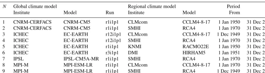
1 CNRM-CERFACS CNRM-CM5 r1i1p1 CLMcom CCLM4-8-17 1 Jan 1950 31 Dec 2100 2 CNRM-CERFACS CNRM-CM5 r1i1p1 SMHI RCA4 1 Jan 1970 31 Dec 2100 3 ICHEC EC-EARTH r12i1p1 CLMcom CCLM4-8-17 1 Dec 1949 31 Dec 2100 4 ICHEC EC-EARTH r12i1p1 SMHI RCA4 1 Jan 1970 31 Dec 2100 5 ICHEC EC-EARTH r1i1p1 KNMI RACMO22E 1 Jan 1950 31 Dec 2100 6 ICHEC EC-EARTH r3i1p1 DMI HIRHAM5 1 Jan 1951 31 Dec 2100 7 IPSL IPSL-CM5A-MR r1i1p1 SMHI RCA4 1 Jan 1970 31 Dec 2100 8 MPI-M MPI-ESM-LR r1i1p1 CLMcom CCLM4-8-17 1 Jan 1970 31 Dec 2100 9 MPI-M MPI-ESM-LR r1i1p1 SMHI RCA4 1 Dec 1949 31 Dec 2100
tures and precipitation on grid cells belonging to the same spatial domain as the observations – i.e. the area of Poland and parts of the Vistula and Odra basins belonging to neigh-bouring countries. This domain corresponds to the area from 13.1 to 26.1◦E and 48.6 to 54.9◦N. The total number of grid cells equalsNg=23 016 (168×137). Selected simula-tions consisted of the combination of four GCMs and four RCMs following the two representative concentration path-ways RCP4.5 and RCP8.5 and are presented in Table 1. We also focused on three common time slices spanning the pe-riod 1971–2000 (referred to hereafter as control pepe-riod) and two future horizons 2021–2050 and 2071–2100 referred to hereafter as near and far future, respectively. As those simu-lations were made available on different spatial resolutions, an interpolation onto the same 5 km×5 km grid as for ob-servations was performed before the bias correction method was applied. For this purpose, we used the nearest-neighbour interpolation method, which means that each cell in the new grid (in this case the 5 km×5 km high resolution) was as-signed the RCM values of the nearest grid cell in their origi-nal grid resolution. We did not correct the interpolated values for altitudinal variations as this was already included in the observational gridded dataset.
3 Data analyses
3.1 Bias correction method
We used the quantile mapping to correct for systematic bi-ases in RCM simulations. The quantile mapping tries to find a statistical transformation or functionF that maps a simu-lated variabley such that its new distribution closely fits the distribution of the observed variablex. In general, this trans-formation can be formulated as
x=F(y). (1)
The non-parametric transformation is then defined as (Piani and Haerter, 2012)
x=F−1(G(y)), (2)
whereGis the cumulative distribution function ofyandF−1
is the inverse cumulative distribution function corresponding
Table 2.RMSEs in annual and seasonal means of monthly sums of precipitation (mm month−1). The RMSEs were computed between historical simulations and observations and averaged over all grid cells.
N GCM/RCM simulation Annual Winter Spring Summer Autumn
1 CNRM-CM5/CCLM4-8-17 13.5 11.7 7.0 45.2 8.5
2 CNRM-CM5/RCA4 15.1 14.5 19.5 27.3 12.2
3 EC-EARTH/CCLM4-8-17 12.6 12.2 8.1 28.5 10.2
4 EC-EARTH/RCA4 14.6 15.8 17.6 24.3 11.4
5 EC-EARTH/RACMO22E 13.1 14.7 13.1 20.3 9.8
6 EC-EARTH/HIRHAM5 19.4 21.7 18.4 22.7 20.9
7 IPSL-CM5A-MR/RCA4 23.2 21.64 33.9 27.3 19.9 8 MPI-ESM-LR/CCLM4-8-17 8.7 13.2 8.7 13.3 10.0
9 MPI-ESM-LR/RCA4 19.4 14.8 26.6 29.1 16.2
Ens. mean∗ All 15.5 15.6 17.0 26.4 13.2
Ens. SD∗ All 4.4 3.7 9.0 8.6 4.7
∗Ens. stands for ensemble, SD for standard deviation.
3.2 Biases in RCM simulations
Each of the nine bias-corrected historical simulations was evaluated on its ability to reproduce statistical properties of the pseudo-observed or reference dataset. In our case, aver-aged error values (e) over time (t) for each grid cell in terms of RMSEs were considered as a measure of the model’s per-formance. As model errors are often seasonally dependent, the four seasons are treated separately. For a timet(seasonal or annual), the model error is calculated as
et=st−ot, (3)
wheres andorefer to simulated and observed values. The RMSE averaged over space is then defined as
RMSE= v u u t 1 Ng Ng X
i=1
e2t, (4)
whereNgis the total number of grid cells.
The averaged RMSE informs about the magnitude of the overall deviation between the simulations and pseudo-observations over all Poland, while the error (e) indicates whether there was an over- (positive) or under- (negative) es-timation (bias) of the simulated values at each grid cell.
The RMSE was computed between values of bias-corrected and raw monthly sums of precipitation, daily min-imum and maxmin-imum temperatures, and their corresponding observations. The model error was first computed on each grid cell, then mapped across Poland and averaged from the spatial field only – i.e. with the RMSE of the temporal means of all grid cells, not of the single grid cells.
Tables 2 to 4 gives the mean and SD of the RMSE derived from the ensemble of model simulations.
The RMSE in annual means averaged over all raw simulations (i.e. multi-model ensemble mean) was 15.5± 4.4 mm month−1for precipitation and 1.1±0.7◦C and 1.6±
0.45◦C for daily minimum and maximum temperatures,
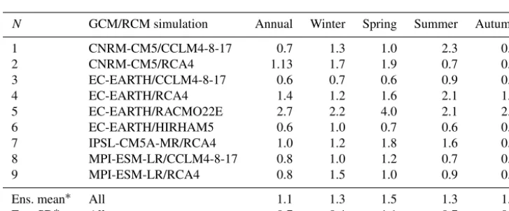
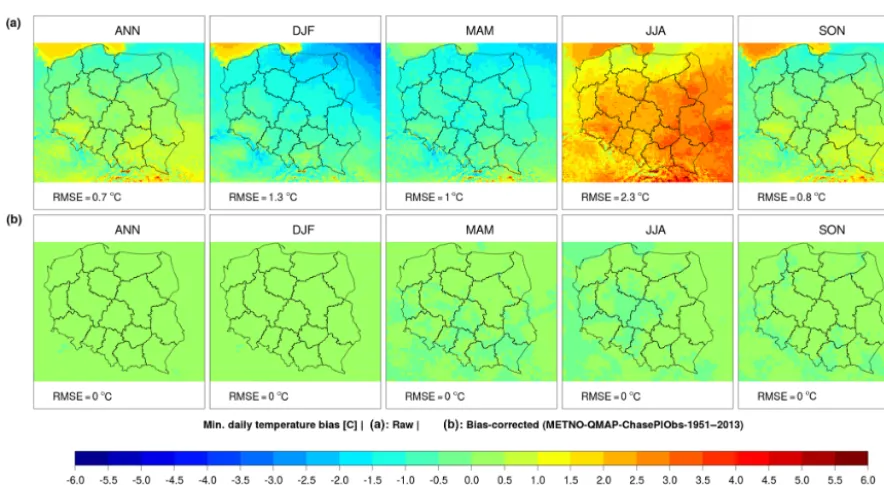
respectively (Tables 2 to 3). For seasonal means, the largest error was found in summer precipitation (26.4± 8.6 mm month−1), mainly due to the convection, not well represented in the climate models. The lowest error was found in the autumn, where precipitation is influenced by continental air masses. The same tendency was additionally found for daily maximum temperature, i.e. large error in the summer compared to the other seasons. However, for daily minimum temperature, the largest error of 1.5◦C was ob-tained for spring, followed by summer with a slightly lower bias of 1.3◦C. In general, biases in daily maximum temper-ature were 0.5 to 1◦C higher than those found in daily min-imum temperature. The lowest precipitation bias was sim-ulated by the regional atmospheric model RCA4 driven by the global model M-MPI-ESM-LR (Simulation 8 in Table 2). Obviously, these biases or model errors might be related to the complexity of the climate system in Poland, which has been very difficult to predict, being influenced by air masses from all four directions (Kundzewicz and Matczak, 2012).
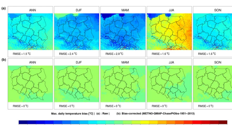
Moreover, model errors or biases are often spatially de-pendant and varied among the simulations and seasons. In our case, all historical simulations showed wet and warm bi-ases as well as dry and cold bibi-ases across the region, which were more pronounced in the mountainous areas located in the southern parts of Poland, due to topographical features not well represented in the models (Figs. 1–27 in the Supple-ment). This can also be related to the low observational net-work density in this region. As we did not intend to perform a thorough comparison between all model simulations, only an example of the bias in the RCM CCLM4-8-17 driven by the CNRM-CM5 GCM for the historical climate (Simulation 1 in Table 1) is detailed here (Figs. 1–3).
Table 3.RMSEs in annual and seasonal means of daily maximum temperature (◦C). RMSEs were computed between historical simulations and observations and averaged over all grid cells.
N GCM/RCM simulation Annual Winter Spring Summer Autumn
1 CNRM-CM5/CCLM4-8-17 1.5 2.4 2.8 1.6 1.6
2 CNRM-CM5/RCA4 1.3 1.6 2.8 1.1 0.6
3 EC-EARTH/CCLM4-8-17 1.6 1.5 1.8 1.6 2.0
4 EC-EARTH/RCA4 1.8 1.1 2.4 2.8 1.3
5 EC-EARTH/RACMO22E 1.9 0.9 2.7 2.7 1.8
6 EC-EARTH/HIRHAM5 2.4 1.5 2.1 3.4 2.8
7 IPSL-CM5A-MR/RCA4 1.7 0.7 3.3 2.8 1.0
8 MPI-ESM-LR/CCLM4-8-17 1.8 1.3 1.4 2.8 1.9
9 MPI-ESM-LR/RCA4 0.8 0.8 0.9 2.1 0.6
Ens. mean∗ All 1.6 1.3 2.3 2.3 1.5
Ens. SD∗ All 0.5 0.5 0.8 0.7 0.7
∗Ens. stands for ensemble, SD for standard deviation.
Table 4.RMSEs in annual and seasonal means of daily minimum temperature (◦C). The RMSEs were computed between historical simula-tions and observasimula-tions and averaged over all grid cells.
N GCM/RCM simulation Annual Winter Spring Summer Autumn
1 CNRM-CM5/CCLM4-8-17 0.7 1.3 1.0 2.3 0.8
2 CNRM-CM5/RCA4 1.13 1.7 1.9 0.7 0.9
3 EC-EARTH/CCLM4-8-17 0.6 0.7 0.6 0.9 0.8
4 EC-EARTH/RCA4 1.4 1.2 1.6 2.1 1.3
5 EC-EARTH/RACMO22E 2.7 2.2 4.0 2.1 2.6
6 EC-EARTH/HIRHAM5 0.6 1.0 0.7 0.6 0.8
7 IPSL-CM5A-MR/RCA4 1.0 1.2 1.8 1.6 0.8
8 MPI-ESM-LR/CCLM4-8-17 0.8 1.0 1.2 0.7 0.8
9 MPI-ESM-LR/RCA4 0.8 1.5 1.0 0.9 0.9
Ens. mean∗ All 1.1 1.3 1.5 1.3 1.1
Ens. SD∗ All 0.7 0.4 1.1 0.7 0.6
∗Ens. stands for ensemble, SD for standard deviation.
wet biases in summer and winter, which were 45.2 and 11.7 mm month−1, respectively, compared to the transition seasons with relatively low biases (7 mm month−1for spring and 8.5 mm month−1 for autumn). The highest discrepancy of the models was obtained in mountainous areas located in the south (negative bias range of−75 to−100 mm month−1) and the eastern part of the region, with a negative bias in the range of−50 to−75 mm month−1. Obviously, the RMSEs from the bias-adjusted results were very low compared to those obtained from the raw simulations and were mostly close to zero for annual and seasonal means – apart from summer, where a small bias of 3.5 mm month−1persisted in the adjusted precipitation. For maximum temperature, there was an overall cold bias for all seasons except for summer, which showed a warm bias everywhere, except for the mountains located in the south exhibiting a more enhanced cold bias. The annual RMSE of the raw data was 1.5◦C. Seasonal evaluations showed higher cold biases for winter
Figure 1.Bias evaluation for Simulation 1 (Table 1). The maps show RMSEs estimated on the difference between historical simulations (all available years included) and observations (CPLFD-GDPT5) for both raw(a)and bias-adjusted(b)monthly sums of precipitation modelled by the CCLM4-8-17 RCM driven by the CNRM-CM5 GCM. The legend “RMSE” indicates the areal mean bias estimated from the gridded annual and seasonal aggregates and the black polylines show the delimitation of the Polish provinces.
Figure 2.As Fig. 1 but for daily maximum temperature.
3.3 Sensitivity to the climate change signal
Although the bias correction significantly improved the qual-ity of the simulations in the trained control time period, it may alter the physical link between climate variables in the
Figure 3.As Fig. 1 but for daily minimum temperature.
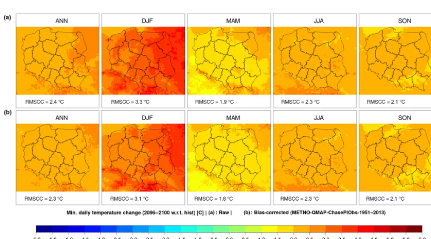
2096–2100 with regard to historical data as we would ex-pect a stronger alteration of the climate signal by the end of the century rather than earlier. An example of results based on the RCM RCA4 driven by the GCM MPI-ESM-LR is illustrated in what follows (Simulation 9 in Table 1). Fig-ures 4–6 suggest that the sign and magnitude and the spatial distribution of the estimated changes were maintained and hence were not affected by the correction procedure. This demonstrated the reliability of the projected climate changes by the corrected RCM simulations. One possible explana-tion could be related to the use of the long reference record (1951–2013) on which the calibration was performed – i.e. the training distribution has been built on a long record en-compassing different climate conditions rather than the short reference periods that are commonly selected (e.g. 1971– 2000 or the new normal, 1981–2010). However, a few ex-ceptions were found. For instance, the magnitude of the cli-mate change (in root mean square terms) between historical and future (2096–2100) simulations for bias-adjusted mod-elled precipitation was reduced by approximately 15 to 25 % in corrected summer and spring changes compared to cor-responding changes in the raw data, respectively, although Hagemann et al. (2005) reported that the impact of the bias correction on the climate change signal may be larger than the signal itself. Overall, the spatial distribution of the cli-mate change signal was, however, consistent in all corrected simulations – i.e. no random effect was introduced by the correction. Similar results were obtained for the other RCM simulations and even when assuming the RCP8.5 scenario (Figs. S28–S54).
4 Projected future climate changes in Poland
The dynamical downscaling performed here involved bias-adjusted RCM simulations taken from the EURO-CORDEX experiment and corrected against the gridded daily dataset CPLFD-GDPT5 (Berezowski et al., 2016). From these datasets, we calculated climatic changes expressed in terms of relative changes in monthly sums of precipitation (in %) and absolute changes in mean temperature (in◦C) with
re-spect to the control period (1971–2000). The mean tempera-ture values were calculated as the average between minimum and maximum temperature values. Although the projections cover small parts lying outside Poland, the maps presented here show only changes over the Polish territory.
We followed a twofold assessment procedure. First, we evaluated the multi-model ensemble means in projecting changes in annual and seasonal means of monthly sums of precipitation and daily means of temperature (Figs. 7 and 8). Second, we focused on projected changes in annual and seasonal means of monthly sums of precipitation and daily minimum and maximum temperatures taken from individual model simulations.
4.1 Changes in the multi-model ensemble mean 4.1.1 Projected temperature changes
spa-Figure 4.Precipitation change signal (mm month−1) for Simulation 9 (Table 1). The maps show absolute changes in the future (2096–2100) with regard to historical simulations (all years included) for both raw(a)and bias-adjusted(b)monthly sums of precipitation modelled by the RCA4 RCM driven by the MPI-ESM-LR GCM. The legend “RMSCC” indicates the areal mean change estimated from the gridded annual and seasonal aggregates and the black polylines show the delimitation of the Polish provinces.
Figure 5.As Fig. 4 but for absolute changes in daily minimum temperature (◦C).
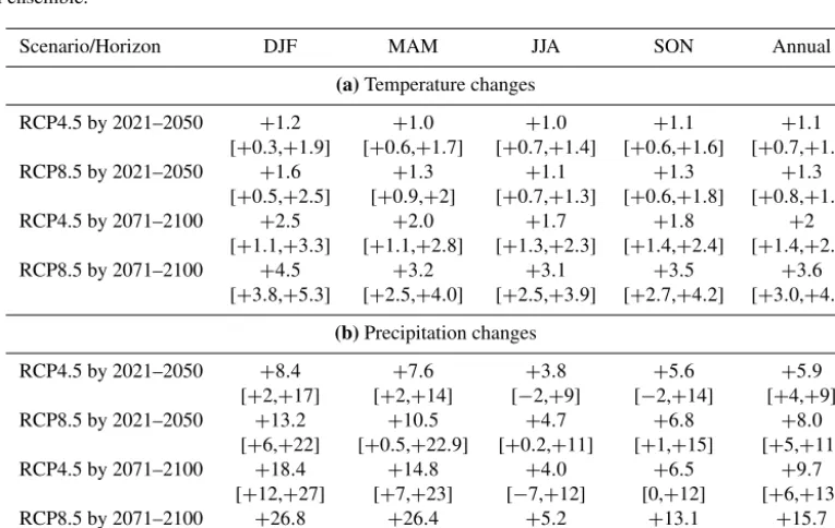
tial variability (the spatial SD is about 0.2◦C; e.g. Fig. 7). On a seasonal basis, the highest change is expected to oc-cur in winter (1.2◦C by 2021–2050 and 2.5◦C by 2071– 2100), followed by spring (1◦C by 2021–2050 and 2◦C by 2071–2100) and autumn (1.1◦C by 2021–2050 and 1.8◦C by
Figure 6.As Fig. 4 but for absolute changes in daily maximum temperature (◦C).
Table 5.Summary of changes in projected multi-model ensemble seasonal and annual regional means of mean temperature (a, in◦C) and precipitation (b, in %) for the near (2021–2050) and far (2071–2100) futures assuming both the RCP4.5 and RCP8.5. Values in brackets indicate the 5th and 95th percentiles of the projected ensembles and hence represent the 90 % confidence interval of the mean estimates from the multi-model ensemble.
Scenario/Horizon DJF MAM JJA SON Annual
(a)Temperature changes
RCP4.5 by 2021–2050 +1.2 +1.0 +1.0 +1.1 +1.1 [+0.3,+1.9] [+0.6,+1.7] [+0.7,+1.4] [+0.6,+1.6] [+0.7,+1.4] RCP8.5 by 2021–2050 +1.6 +1.3 +1.1 +1.3 +1.3
[+0.5,+2.5] [+0.9,+2] [+0.7,+1.3] [+0.6,+1.8] [+0.8,+1.8] RCP4.5 by 2071–2100 +2.5 +2.0 +1.7 +1.8 +2
[+1.1,+3.3] [+1.1,+2.8] [+1.3,+2.3] [+1.4,+2.4] [+1.4,+2.5] RCP8.5 by 2071–2100 +4.5 +3.2 +3.1 +3.5 +3.6
[+3.8,+5.3] [+2.5,+4.0] [+2.5,+3.9] [+2.7,+4.2] [+3.0,+4.1]
(b)Precipitation changes
RCP4.5 by 2021–2050 +8.4 +7.6 +3.8 +5.6 +5.9 [+2,+17] [+2,+14] [−2,+9] [−2,+14] [+4,+9] RCP8.5 by 2021–2050 +13.2 +10.5 +4.7 +6.8 +8.0
[+6,+22] [+0.5,+22.9] [+0.2,+11] [+1,+15] [+5,+11] RCP4.5 by 2071–2100 +18.4 +14.8 +4.0 +6.5 +9.7
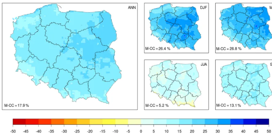
[+12,+27] [+7,+23] [−7,+12] [0,+12] [+6,+13] RCP8.5 by 2071–2100 +26.8 +26.4 +5.2 +13.1 +15.7
[+18,+35] [+16,+39] [−5,+15] [−1,+25] [+9,+23]
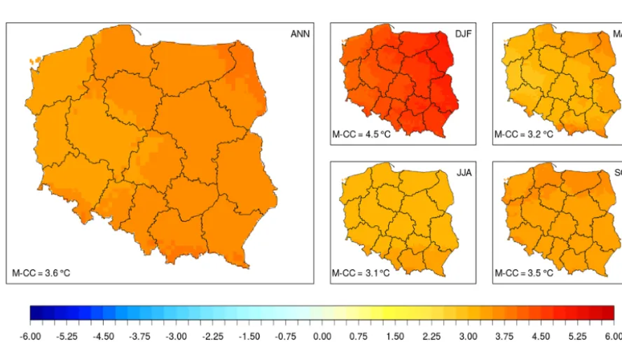
The warming rate is accelerated when assuming the RCP8.5 emission scenario and when the far future time hori-zon is considered (Table 5a). As in the RCP4.5 scenario, the warming is expected to be highest during the winter season and the mean temperature is likely to be 4.5◦C across the
re-Figure 7.Projected temperature changes (◦C) for the far future (2071–2100) assuming the RCP4.5 scenario. Maps show annual(a)and seasonal(b)changes in the multi-model ensemble mean of absolute temperature with regard to the control period (1971–2000). The legend “M-CC” means the areal mean change estimated from the gridded data.
Figure 8.As Fig. 7 but for projected temperature changes (◦C) in the far future (2071–2100) assuming the RCP8.5 scenario.
gions in the south, where temperatures are expected to rise by as much as 3◦C by 2071–2100.
4.1.2 Projected precipitation changes
Projections show that Poland is expected to get more precip-itation in the future in all seasons (Table 5b). In general, the
projections based on the two scenarios show similar changes for the near future. But for the far future, the RCP8.5 high-emission scenario projects a significantly stronger increase.
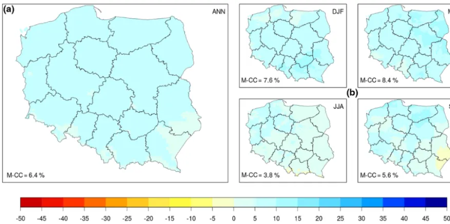
Figure 9.Projected changes in monthly sums of precipitation (%) for the period (2021–2050) assuming the RCP4.5 scenario. Maps show annual(a)and seasonal(b)changes in the multi-model ensemble mean of absolute temperature with regard to the control period (1971–2000). The legend “M-CC” means the areal mean change estimated from the gridded data.
and 10 % by the far future (2071–2100). On a seasonal basis, the highest rates are expected to occur in winter (+8 % by 2021–2050 and+18 % by 2071–2100) and spring (+8 % by 2021–2050 and +15 % by 2071–2100), while the smallest changes are expected to occur in summer (+4 % for both fu-ture time periods) and autumn (+6 to+7 %, regardless of the future period). Those projected changes are in line with Ro-manowicz et al. (2016), who found a precipitation increase of up to 15 % considering only 10 small catchments spread across the country (not for all of Poland).
Assuming the RCP8.5 scenario, the expected change by the far future (2071–2100) is approximately +16 % for the annual mean precipitation, with stronger increases in win-ter (27 %) and spring (26 %), and more moderate changes in summer (+5 %) and autumn (+13 %). Summer exhibits sim-ilar changes in precipitation regardless of emission scenario and time horizon.
In contrast to temperature, precipitation changes reveal higher variability in space (spatial SD averaged across all scenarios and periods equals 5 %). In southern Poland, north of the Carpathian Mountains, summer and autumn precip-itation are even expected to decrease by as much as 5 % (Fig. 9). The influenced area is more pronounced in projec-tions for the far future (2071–2100) and when assuming the high-emission scenario RCP8.5 (Fig. 10).
4.2 Changes in individual model simulations
4.2.1 Projected temperature changes
Results based on bias-adjusted individual model simulations also show a systematic increase in both minimum and max-imum temperatures for the two future periods and RCPs, re-spectively.
Assuming the RCP4.5 scenario, the absolute changes in annual means of daily minimum temperature by 2021–2050 vary between 0.8 and 1.6◦C (Fig. S83). On a seasonal ba-sis, the warming is more intensified in winter (Fig. 11), varying from 0.3◦C (CCLM4-8-17/MPI-ESM-LR) to 2.2◦C (HIRAM5/EC-EARTH), and slightly amplified in spring (Fig. S91), varying from 0.7 to 1.8◦C, respectively. Al-though changes in annual means of daily maximum tem-perature are expected to have similar magnitude, they are slightly less pronounced than for daily minimum temperature and vary from 0.6 to 1.4◦C. The same tendency was found for seasonal means of maximum temperature, which exhibit a slightly amplified magnitude in autumn when compared to seasonal means of daily minimum temperature, and vary be-tween 0.5 and 1.6◦C (Fig. S119). The lowest increase is
Figure 10.As Fig. 9 but for projected precipitation changes (%) by 2071–2100 assuming RCP8.5 scenario.
the highest projected warming is expected to reach approx-imately 3◦C. The autumn and summer means of daily min-imum temperature show the same amplitude as the annual changes, and vary from 1.5 to 2.5◦C and 1.4 to 2.5◦C, re-spectively. Likewise, the changes in seasonal means of maxi-mum temperature range from 1.2 to 3.2◦C in winter, from 0.9 to 2.9◦C in spring, from 1.3 and 2.7◦C in autumn, and from 1◦C to 2.4◦C in summer (Supplement Sect. 4.2). Again, summer means of daily maximum temperature exhibit the lowest warming. Similarly to precipitation, both temperature variables show large differences between the simulations in projecting the magnitude of the seasonal changes. However, they all agree on the sign of the change (e.g. Fig. S104 and S112).
When assuming the RCP8.5 scenario, changes in annual means of minimum (Fig. S85) and maximum (Fig. S105) temperature show slightly higher increases by as much as 0.5 and 0.25◦C in the near future time period, respectively, than what is expected when assuming the RCP4.5 scenario. These increases are expected to be more amplified by 2◦C by the end of the 21st century (Fig. S86 and S106). The high-est warming is expected to occur in winter means of daily minimum temperature with an increasing rate higher than 5◦C simulated by the RCA4 and CCLM4-8-17 RCMs, both driven by the CNRM-CM5 GCM (Fig. S90).
Piniewski et al. (2017a) assessed the robustness of the tem-perature change signal using the same set of RCM simula-tions and demonstrated that the increase obtained in the an-nual means of daily minimum and maximum temperature was robust. However, a lower robustness was found on the seasonal scale.
4.2.2 Projected precipitation changes
gra-Figure 11.Changes in projected winter means of daily minimum temperature by 2021–2050 assuming the RCP4.5 scenario. The maps show the absolute changes with regard to the historical period (1971–2000) for all nine adjusted simulations.
dient is reproduced. For the spring season (Fig. S71), there is a dominance of mostly wet patterns, where precipitation changes vary from +1 % (CCLM4-8-17/CNRM-CM5 sim-ulation) to+17 % (CCLM4-8-7/MPI-ESM-LR simulation). Similarly, autumn precipitation changes are expected to vary between −4 and 13 % and show similar patterns to those obtained for winter. Hence, no agreement between the cor-rected simulations was seen for the near future (Fig. S79). The direction of the change signal becomes clearer towards the end of the century, showing overall wetter conditions on an annual scale, and the projected changes are expected to vary from 4 % (RCA4/MPI-ESM-LR simulation) to 13 % (RCA4/CNRM-CM5 simulation) (Fig. SM 60). Surprisingly,
Figure 12.Changes in projected annual means of monthly sums of precipitation by 2021–2050 assuming the RCP4.5 scenario. The maps show relative changes with regard to the historical time period (1971–2000) for the nine bias-adjusted simulations.
the CCLM4-18-17 RCM driven by the EC-EARTH GCM, and they are more robust in spring than in winter.
Assuming the RCP8.5 scenario, the spatial distribution of the increase in the annual means of precipitation becomes more dominant, and results show rather good agreement between simulations on projected wetter conditions by as much as 22 % (Fig. S65–S66), except for the HIRHAM5/EC-EARTH simulation, which shows a decrease of less than 5 % by the near future in southwestern areas (Fig. S65). In general, this amplification can be due to the increase in wa-ter vapour associated with warmer future climate conditions. The same annual tendency is reflected in winter and spring, but the magnitude of the change varies much between the
simulations (+14 to+41 %). In summer and autumn, how-ever, the disagreement in the projected climate change sig-nal persists to the end of the century, during which wetter and drier conditions are likely to occur (Fig. 14). For in-stance, the RCA4 RCM driven by the EC-EARTH GCM projects a decrease in summer precipitation down to 6 %, whereas the CCLM4-8-17 RCM driven by the CNRM-CM5 GCM shows overall wet patterns and an increase of up to 15 %. The largest increase in winter is projected by the RACMO22E/EC-EARTH simulation (Fig. 15).
Figure 13.Changes in projected summer means of monthly sums of precipitation by 2021–2050 assuming the RCP4.5 scenario. The maps show the relative changes with regard to the historical period (1971–2000) for the nine adjusted simulations.
the changes were, in general, uncertain and not robust. They also pointed out that the spatial variability of the climate change signal was quite variable between individual climate model simulations, which considerably reduced the robust-ness, especially for the far future.
5 Data availability
The CHASE-PL Climate Projection (CPLCP) dataset pro-duced here was made available for use in two different ways: (1) in a long-lasting research data repository and (2) through a dedicated CHASE-PL web geoportal. The first option (Sect. 5.1) is meant to serve mainly researchers, particularly
Figure 14.Changes in projected summer means of monthly sums of precipitation by 2071–2100 assuming the RCP8.5 scenario. The maps show the relative changes with regard to the historical period (1971–2000) for the nine adjusted simulations.
5.1 Data repository at 4TU.Centre for Research Data
The bias-adjusted files were stored in NetCDF4 format and compiled using the Climate and Forecast (CF) conventions. The data were made available at the 4TU.Centre for Re-search Data (Mezghani et al., 2016). The files consist of nine bias-adjusted RCM simulations of daily (minimum and maximum) temperature and precipitation for a spatial do-main covering the union of Poland and the Vistula and Odra basins for one historical and two future time periods as-suming the RCP4.5 and RCP8.5 scenarios. There are 135 files and the total size is 127 GB. The full dataset cov-ering the continuous time period (i.e. 1950–2100) can be obtained upon request from the Norwegian
Meteorologi-cal Institute. The CPLCP-GDPT5 dataset presented here is publicly available at https://doi.org/10.4121/uuid:e940ec1a-71a0-449e-bbe3-29217f2ba31d.
Figure 15.Changes in projected winter means of monthly sums of precipitation by 2071–2100 assuming the RCP8.5 scenario. The maps show the relative changes with regard to the historical period (1971–2000) for all nine adjusted simulations.
monthly/seasonal/annual time series and long-term average values. The “Impacts” sub-page presents maps of climate change impacts on water resources (Piniewski et al., 2017b) obtained from hydrological modelling using SWAT driven by the dataset described in this paper. In this section we focus on the “Projections” sub-page presenting the contents of the CHASE-PL Climate Projections dataset (Fig. 16).
The web-map application was developed using ArcGIS Server, which makes the data available using REST archi-tecture, as well as using the temporal data visualization por-tal using the JavaScript API for communication between the client and the server. ESRI Geoportal Server was applied for meta-data management. Two language versions, English and
Figure 16.Example of the “Projections” sub-page of the Climate Impact Geoportal http://climateimpact.sggw.pl. The maps show the ensem-ble median change in mean annual and seasonal precipitation following RCP8.5 in the far future, and the popup window displays interactive values for a selected grid cell from the map.
the spread of change (climate model uncertainty). The web-map application has the following functionalities: (1) meta-data searching, (2) searching by location, (3) identification of selected values on the map (simultaneously for all seasons and year), and (4) data download in NetCDF and GeoTIFF formats. The online help and glossary were also created in order to enhance the use of the geoportal among users less advanced in web GIS and/or climate model outputs.
6 Conclusions
A recent high-resolution gridded dataset (CHASE-PL Forc-ing Data “CPLFD-GDPT5”) was used as long-term refer-ence dataset produced over the Odra and Vistula basins in Poland and surrounding regions to correct for any system-atic bias in daily precipitation and temperatures simulated by nine EURO-CORDEX RCMs. The main purpose was to pro-vide up-to-date climate projections for Poland assuming the new generation of representative concentration pathways.
Results showed that the bias correction method performed very well in reducing the large biases found in the raw data of an ensemble of nine EURO-CORDEX simulations.
Regarding the climate projections, we demonstrated that the climate change signal was not affected by the bias cor-rection method. Yet, any misrepresentation of the former in the RCM, due, for instance, to inherited misrepresentation of (i) the sea surface temperatures and sea ice extent in the northern parts influenced by the Baltic Sea and (ii) topo-graphical features (e.g. the mountains located in the southern parts) could have an influence on the projected temperature and precipitation changes (Wibig et al., 2015). Nevertheless,
we assumed that changes in the climate parameters were less affected than their absolute values and hence showed more robust estimates.
Based on the best estimates, projected changes in tem-perature and precipitation suggest a warmer and wetter cli-mate over Poland for the coming decades, except for sum-mer, during which a decrease in precipitation by less than 7 % is also likely to occur. The warming over Poland is ex-pected to likely vary by 0.3◦C by 2021–2050 assuming the intermediate-emission scenario. This accelerates to approx-imately 5◦C towards the end of the 21st century assuming the high-emission scenario. Similarly to temperature, precip-itation over Poland is expected to vary by between−7 and +40 %. The highest increases in both temperature and pre-cipitation are expected to occur in winter.
We believe that the CHASE-PL Climate Projection prod-uct (CPLCP-CPLFD-GDPT5) available for the period of 150 years (from 1951 to 2100) will serve as the basis for further applications – for instance, to study the impact of cli-mate change over Poland on many sectors (e.g. agriculture, hydrology, ecology, and tourism).
The Supplement related to this article is available online at https://doi.org/10.5194/essd-9-905-2017-supplement.
Competing interests. The authors declare that they have no con-flict of interest.
Acknowledgements. We acknowledge the Polish–Norwegian
Research Programme operated by the National Centre for Research and Development (NCBiR) under the Norwegian Financial Mech-anism 2009–2014 for financial support of the project CHASE-PL (Climate change impact assessment for selected sectors in Poland) in the framework of project contract no. Pol-Nor/200799/90/2014 and the World Climate Research Programme’s Working Group on Regional Climate, and the Working Group on Coupled Modelling, former coordinating body of CORDEX and responsible panel for CMIP5. We also thank the climate modelling groups (listed in Table 1 of this paper) for producing and making available their model output. We also acknowledge the Earth System Grid Federation infrastructure – an international effort led by the US Department of Energy’s Program for Climate Model Diagnosis and Intercomparison, the European Network for Earth System Modelling, and other partners in the Global Organization for Earth System Science Portals (GO-ESSP). Co-author M. Piniewski is additionally grateful for support from the Alexander von Humboldt Foundation and the Ministry of Science and Higher Education of the Republic of Poland. Finally, we would like to thank the two reviewers, Joanna Wibig and Mirosław Mie¸tus, for their respective positive and constructive comments that helped to improve the paper.
Edited by: David Carlson
Reviewed by: Joanna Wibig and Mirosław Mie¸tus
References
Benestad, R. E., Achberger, C., and Fernandez, E.: Empirical-statistical downscaling of distribution functions for daily precip-itation, Climate 12/2005, The Norwegian Meteorological Insti-tute, Oslo, Norway, http://www.met.no, 2005.
Berezowski, T., Szcze´sniak, M., Kardel, I., Michałowski, R., Okruszko, T., Mezghani, A., and Piniewski, M.: CPLFD-GDPT5: High-resolution gridded daily precipitation and tem-perature data set for two largest Polish river basins, Earth Syst. Sci. Data, 8, 127–139, https://doi.org/10.5194/essd-8-127-2016, 2016.
Berg, P., Feldmann, H., and Panitz, H. J.: Bias correction of high resolution regional climate model data, J. Hydrol., 448–449, 80– 92, https://doi.org/10.1016/j.jhydrol.2012.04.026, 2012. Boé, J., Terray, L., Habets, F., and Martin, E.: Statistical
and dynamical downscaling of the Seine basin climate for hydro-meteorological studies, Int. J. Climatol., 27, 1643–1655, https://doi.org/10.1002/joc.1602, 2007.
Buishand, A. and Beckmann, B.: Development of Daily Precipita-tion Scenarios at KNMI, Tech. Rep., ECLAT-2 Workshop Report No. 3, Royal Netherlands Meteorological Institute, De Bilt, the Netherlands, 2000.
Buishand, T. A. and Brandsma, T.: Comparison of circulation clas-sification schemes for predicting temperature and precipitation in the Netherlands, Int. J. Climatol., 17, 875–889, 1997.
Buishand, T. A. and Brandsma, T.: Multisite simulation of daily pre-cipitation and temperature in the Rhine basin by nearest-neighbor resampling, Water Resour. Res., 37, 2761–2776, 2001.
Chen, J., Brissette, F. P., Chaumont, D., and Braun, M.: Finding appropriate bias correction methods in downscaling precipitation for hydrologic impact studies over North America, Water Resour. Res., 49, 4187–4205, https://doi.org/10.1002/wrcr.20331, 2013. Christensen, J. H., Boberg, F., Christensen, O. B., and
Lucas-Picher, P.: On the need for bias correction of regional climate change projections of temperature and precipitation, Geophys. Res. Lett., 35, L20709, https://doi.org/10.1029/2008GL035694, 2008.
Déqué, M., Rowell, D. P., Lüthi, D., Giorgi, F., Christensen, J. H., Rockel, B., Jacob, D., Kjellström, E., Castro, M. d., and Hurk, B. v. d.: An intercomparison of regional climate simulations for Europe: assessing uncertainties in model projections, Climatic Change, 81, 53–70, https://doi.org/10.1007/s10584-006-9228-x, 2007.
Ehret, U., Zehe, E., Wulfmeyer, V., Warrach-Sagi, K., and Liebert, J.: HESS Opinions “Should we apply bias correction to global and regional climate model data?”, Hydrol. Earth Syst. Sci., 16, 3391–3404, https://doi.org/10.5194/hess-16-3391-2012, 2012. Fang, G. H., Yang, J., Chen, Y. N., and Zammit, C.: Comparing bias
correction methods in downscaling meteorological variables for a hydrologic impact study in an arid area in China, Hydrol. Earth Syst. Sci., 19, 2547–2559, https://doi.org/10.5194/hess-19-2547-2015, 2015.
Fowler, H. J. and Kilsby, C. G.: Using regional climate model data to simulate historical and future river flows in northwest England, Climatic Change, 80, 337–367, 2007.
Giorgi, F. and Lionello, P.: Climate change projections for the Mediterranean region, Global Planet. Change, 63, 90–104, https://doi.org/10.1016/j.gloplacha.2007.09.005, 2008.
Gudmundsson, L., Bremnes, J. B., Haugen, J. E., and Engen-Skaugen, T.: Technical Note: Downscaling RCM precipitation to the station scale using statistical transformations – a com-parison of methods, Hydrol. Earth Syst. Sci., 16, 3383–3390, https://doi.org/10.5194/hess-16-3383-2012, 2012.
Haerter, J. O., Hagemann, S., Moseley, C., and Piani, C.: Climate model bias correction and the role of timescales, Hydrol. Earth Syst. Sci., 15, 1065–1079, https://doi.org/10.5194/hess-15-1065-2011, 2011.
Hagemann, S., Arpe, K., and Bengtsson, L.: Validation of the hy-drological cycle of ERA-40, ERA-40 Project Report Series 24, ECMWF, http://www.ecmwf.int, Reading, UK, 2005.
Ines, A. V. and Hansen, J. W.: Bias correction of daily GCM rainfall for crop simulation studies, Agr. Forest Meteorol., 138, 44–53, https://doi.org/10.1016/j.agrformet.2006.03.009, 2006.
Kundzewicz, Z. W. and Matczak, P.: Climate change regional re-view: Poland: climate change regional rere-view: Poland, WIREs Clim. Change, 3, 297–311, https://doi.org/10.1002/wcc.175, 2012.
Lafon, T., Dadson, S., Buys, G., and Prudhomme, C.: Bias cor-rection of daily precipitation simulated by a regional climate model: a comparison of methods, Int. J. Climatol., 33, 1367– 1381, https://doi.org/10.1002/joc.3518, 2013.
ap-plications to historical radiosonde station data, Int. J. Climatol., 16, 1197–1226, 1996.
Linden, P. v. d. and Mitchell, J. F. B.: Ensembles: Climate Change and its impacts: summary of research and results from the EN-SEMBLES project, European Comission, Met Office Hadley Centre, Exeter, UK, 2009.
Mezghani, A., Dobler, A., and Haugen, J.: CHASE-PL Cli-mate Projections–Gridded Daily Precipitation and Tem-perature Dataset at 5 km resolution for Poland, Norwe-gian Meteorological Institute, Oslo, Norway, Dataset, https://doi.org/10.4121/uuid:e940ec1a-71a0-449e-bbe3-29217f2ba31d, 2016.
Muerth, M. J., Gauvin St-Denis, B., Ricard, S., Velázquez, J. A., Schmid, J., Minville, M., Caya, D., Chaumont, D., Lud-wig, R., and Turcotte, R.: On the need for bias correction in regional climate scenarios to assess climate change im-pacts on river runoff, Hydrol. Earth Syst. Sci., 17, 1189–1204, https://doi.org/10.5194/hess-17-1189-2013, 2013.
Osuch, M., Kindler, Romanowicz, R. J., Berbeka, K., and Ban-rowska, A.: KLIMADA Strategia adaptacji Polski do zmian kli-matu w zakresie sektora “Zasoby i gospodarka wodna”, Tech. rep., KLIMADA project, IGF PAN, Warsaw, 245 pp., 2012. Osuch, M., Romanowicz, R. J., Lawrence, D., and Wong, W. K.:
Trends in projections of standardized precipitation indices in a future climate in Poland, Hydrol. Earth Syst. Sci., 20, 1947– 1969, https://doi.org/10.5194/hess-20-1947-2016, 2016. Piani, C. and Haerter, J. O.: Two dimensional bias correction of
tem-perature and precipitation copulas in climate models, Geophys. Res. Lett., 39, L20401, https://doi.org/10.1029/2012GL053839, 2012.
Piniewski, M., Mezghani, A., Szcze´sniak, M., and Kundzewicz, Z. W.: Regional projections of temperature and precipitation changes: robustness and uncertainty aspects, Meteorol. Z., 26, 223–234, https://doi.org/10.1127/metz/2017/0813, 2017a. Piniewski, M., Szcze´sniak, M., Huang, S., and Kundzewicz, Z. W.:
Projections of runoff in the Vistula and the Odra river basins with the help of the SWAT model, Hydrol. Res., 48, nh2017280, https://doi.org/10.2166/nh.2017.280, 2017b.
Piotrowski, P. and Je¸druszkiewicz, J.: Projections of ther-mal conditions for Poland for winters 2021-2050 in rela-tion to atmospheric circularela-tion, Meteorol. Z., 22, 569–575, https://doi.org/10.1127/0941-2948/2013/0450, 2013.
Pluntke, T., Schwarzak, S., Kuhn, K., Lünich, K., Adynkiewicz-Piragas, M., Otop, I., and Miszuk, B.: Climate analy-sis as a baanaly-sis for a sustainable water management at the Lusatian Neisse, Meteorology Hydrology and Water Management, Research and Operational Applications, 4, 3–11, https://www.infona.pl//resource/bwmeta1.element. baztech-d8873b7d-b425-414a-9dbe-8451e1ca46f3, 2016. Romanowicz, R. J., Bogdanowicz, E., Debele, S. E.,
Doroszkiewicz, J., Hisdal, H., Lawrence, D., Meresa, H. K., Napiórkowski, J. J., Osuch, M., Strupczewski, W. G., Wilson, D., and Wong, W. K.: Climate change im-pact on hydrological extremes: preliminary results from the Polish-Norwegian Project, Acta Geophys., 64, 477–509, https://link.springer.com/article/10.1515/acgeo-2016-0009, 2016.
Sorteberg, A., Haddeland, I., Haugen, J. E., Sobolowski, S., and Wong, W. K.: Evaluation of distribution mapping based bias cor-rection methods, Tech. Rep., Norwegian Centre for Climate Ser-vices (NCCS), Oslo, Norway, Report no. 1/2014, pp. 23, 2014. Szwed, M., Karg, G., Pi´nskwar, I., Radziejewski, M., Graczyk, D.,
Ke¸dziora, A., and Kundzewicz, Z. W.: Climate change and its effect on agriculture, water resources and human health sec-tors in Poland, Nat. Hazards Earth Syst. Sci., 10, 1725–1737, https://doi.org/10.5194/nhess-10-1725-2010, 2010.
Teng, J., Potter, N. J., Chiew, F. H. S., Zhang, L., Wang, B., Vaze, J., and Evans, J. P.: How does bias correction of regional climate model precipitation affect modelled runoff?, Hydrol. Earth Syst. Sci., 19, 711–728, https://doi.org/10.5194/hess-19-711-2015, 2015.
Teutschbein, C. and Seibert, J.: Bias correction of regional climate model simulations for hydrological climate-change impact stud-ies: review and evaluation of different methods, J. Hydrol., 456, 12–29, https://doi.org/10.1016/j.jhydrol.2012.05.052, 2012. Themeßl, M. J., Gobiet, A., and Leuprecht, A.: Empirical-statistical
downscaling and error correction of daily precipitation from re-gional climate models, Int. J. Climatol., 31, 1530–1544, 2010. Wibig, J., Maraun, D., Benestad, R., Kjellström, E., Lorenz,