Performance evaluation of a throughput-aware framework for ensemble data assimilation: the case of NICAM-LETKF

(1)

www.geosci-model-dev.net/9/2293/2016/ doi:10.5194/gmd-9-2293-2016

Performance evaluation of a throughput-aware framework for

ensemble data assimilation: the case of NICAM-LETKF

Hisashi Yashiro1, Koji Terasaki1, Takemasa Miyoshi1,2,3, and Hirofumi Tomita1

1_{RIKEN Advanced Institute for Computational Science, Kobe, Japan}

2_{Application Laboratory, Japan Agency for Marine-Earth Science and Technology, Yokohama, Japan} 3_{University of Maryland, College Park, Maryland, USA}

Correspondence to:Hisashi Yashiro ([email protected])

Received: 8 January 2016 – Published in Geosci. Model Dev. Discuss.: 12 February 2016 Revised: 30 May 2016 – Accepted: 17 June 2016 – Published: 5 July 2016

Abstract. In this paper, we propose the design and imple-mentation of an ensemble data assimilation (DA) framework for weather prediction at a high resolution and with a large ensemble size. We consider the deployment of this frame-work on the data throughput of file input/output (I/O) and multi-node communication. As an instance of the applica-tion of the proposed framework, a local ensemble transform Kalman filter (LETKF) was used with a Non-hydrostatic Icosahedral Atmospheric Model (NICAM) for the DA sys-tem. Benchmark tests were performed using the K com-puter, a massive parallel supercomputer with distributed file systems. The results showed an improvement in total time required for the workflow as well as satisfactory scalabil-ity of up to 10 K nodes (80 K cores). With regard to high-performance computing systems, where data throughput formance increases at a slower rate than computational per-formance, our new framework for ensemble DA systems promises drastic reduction of total execution time.

1 Introduction

Rapid advancements in high-performance computing (HPC) resources in recent years have enabled the development of at-mospheric models to simulate and predict the weather at high spatial resolution. For effective use of massive parallel super-computers, parallel efficiency becomes a common but critical issue in weather and climate modeling. Scalability for sev-eral large-scale simulations has been accomplished to a cer-tain extent thus far. For example, the Community Earth Sys-tem Model (CESM) performs high-resolution coupled

cli-mate simulations by using over 60 K cores of an IBM Blue Gene/P system (Dennis et al., 2012). Miyamoto et al. (2013) generated the first global sub-kilometer atmosphere simula-tion by using the Non-hydrostatic Icosahedral Atmospheric Model (NICAM) with 160 K cores of the K computer.

Climate simulations at such high resolutions need to be able to handle the massive amounts of input/output (hence-forth, I/O) data. Since the throughput of file I/O is much lower than that of the main memory, I/O performance is important to maintaining the scalability of the simulations as well as guaranteeing satisfactory computational perfor-mance. Parallel I/O is necessary to improve the total through-put of I/O. In order to improve performance, a few li-braries have been developed for climate models, e.g., the application-level parallel I/O (PIO) library, which was de-veloped (Dennis et al., 2011) and applied to each compo-nent model of the CESM. The XML I/O server (XIOS, http: //forge.ipsl.jussieu.fr/ioserver) was used in European models, such as EC-EARTH (Hazeleger et al., 2010). XIOS distin-guishes the I/O node group from the simulation node group and asynchronously transfers data for output generated by the latter group to the former. With the development of models at increasing spatial resolution, the use of parallel I/O libraries will become more common.

(2)

fil-ter (EnKF, Evensen, 1994, 2003) – are used at operational forecasting centers. Hybrid ensemble/4D-Var systems have also been recently developed (Clayton et al., 2013). 4D-Var systems require an adjoint model that relies heavily on the simulation model. By contrast, DA systems using the EnKF method are independent of the model. Ensemble size is a critical factor in obtaining statistical information regarding the simulated state in an ensemble DA system. Miyoshi et al. (2014, 2015) performed 10 240-member EnKF experi-ments and proposed that the typical choice of an ensemble size of approximately 100 members is insufficient to capture the precise probability density function and long-range error correlations. Thus, it is reasonable to increase not only the resolution of the model, but also its ensemble size in accor-dance with performance enhancement yielded by supercom-puters. However, this enhancement in model resolution and ensemble size leads to a tremendous increase in total data in-put and outin-put. For example, prevalent DA systems operating at high resolution with a large number of ensemble members require terabyte-scale data transfer between components. In the future, the volume of data in large-scale ensemble DA systems is expected to reach the petabyte scale.

In such cases, data movement between the simulation model and the ensemble DA systems will become the most significant issue. This is because data distribution patterns for inter-node parallelization in the two systems are differ-ent. The processes of a simulation model share all global grids of a given ensemble member. By contrast, the DA sys-tem requires all ensemble members for each process. Even if the simulation model and the DA system use the same pro-cesses, the data layout in each is different and, hence, needs to be altered between them. Thus, a large amount of data exchange through inter-node communication or file I/O is re-quired. This problem needs to be addressed in order to en-hance the scalability of the ensemble DA system.

As described above, data throughput between model simu-lations and ensemble DA systems becomes much larger than that for single atmospheric simulations. We are now con-fronted with the problem of data movement between the two components. Hamrud et al. (2015) have pointed out the lim-itation of scaling by using file I/O in the European Cen-tre for Medium-range Weather Forecasts’ (ECMWF) semi-operational ensemble Kalman filter (EnKF) system. By con-trast, Houtekamer et al. (2014) showed satisfactory scalabil-ity in a Canadian operational EnKF DA system by using par-allel I/O. This study aims to investigate the performance of ensemble DA systems by focusing on reducing data move-ment. NICAM (Satoh et al., 2014) and a local ensemble transform Kalman filter (LETKF) (Hunt et al., 2007) were used as reference cases for the model and the DA system, respectively. In Sect. 2, we summarize the design and imple-mentation of the conventional framework for ensemble DA systems, and illuminate the problem from the perspective of data throughput. To solve the problem, we propose our framework for DA systems in Sect. 3. In order to test the

ef-fectiveness of our framework, we describe performance and scalability in the case of NICAM and LETKF on the K com-puter, which has a typical mesh torus topology for inter-node communication, in Sect. 4. We summarize and discuss the results in Sect. 5.

2 NICAM–LETKF DA system

NICAM (Satoh et al., 2014) is a global non-hydrostatic at-mospheric model developed mainly at the Japan Agency for Marine-Earth Science and Technology, University of Tokyo, and the RIKEN Advanced Institute for Computa-tional Science. With the aid of state-of-the-art supercomput-ers, NICAM has been contributing to atmospheric model-ing at high resolutions. The first global simulations with a 3.5 km horizontal mesh were carried out on the Earth Sim-ulator. The simulations showed a realistic multi-scale cloud structure (Tomita, 2005; Miura et al., 2007). The K computer allowed many more simulations at the same or higher reso-lutions. Miyakawa et al. (2014) showed using several case studies that the skill score of the Madden–Julian Oscilla-tion (MJO) (Madden and Julian, 1972) improved by using a convection-resolving model in comparison with other mod-els. As a climate simulation, the 30-year AMIP-type simula-tion was conducted with a 14 km horizontal mesh (Kodama et al., 2015). The global sub-kilometer simulation revealed that the essential change in convection statistics occurred at a grid spacing of approximately 2 km (Miyamoto et al., 2013). NICAM employs fully compressible non-hydrostatic dynam-ics where the finite volume method is used for discretiza-tion on the icosahedral grid system. The grid point method has the advantage of reducing data transfer between compu-tational nodes over a spectral transform method, which re-quires global communication between nodes and constitutes one of the bottlenecks in a massively parallel machine.

(3)

separately executed for each grid. The NICAM–LETKF sys-tem is based on the code for the LETKF by Miyoshi (2005). Miyoshi and Yamane (2007) applied a parallel algorithm to the LETKF for efficient parallel computation, and Miyoshi et al. (2010) addressed load imbalance in the algorithm.

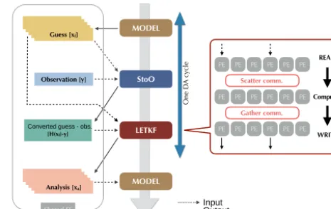
The following is devoted to an explanation of the current NICAM-LETKF and a clarification of the problem. Figure 1 shows a flow diagram of the DA system with the LETKF and an atmospheric model. In this DA system, three applica-tion programs are used: an atmospheric simulaapplica-tion model, a simulation-to-observation converter (henceforth, StoO), and the LETKF. These programs are executed sequentially in a DA cycle. Most atmospheric models often use aggregated data for file I/O. This framework also assumes that each member has only a single file containing the simulated state. The numbers of computational nodes to be used are sepa-rately set for each program component. Since no component contains knowledge of the process used for file I/O, the out-put should be located in the shared file system; otherwise, the components cannot share information with one another. The StoO program reads the simulation results [Xf] and

obser-vation data [y] as a first guess. The simulation results are di-agnostically converted into observed variables [H (xf)]. By

using information regarding the horizontal and vertical lo-cations, the model grid data are interpolated to data at the position of observation. Variable conversions, such as radia-tion calcularadia-tions, are also applied when necessary. Following the conversion, the difference between the converted sim-ulation results and the observations [H (xf)−y] is

calcu-lated for the output. The StoO program is independently ex-ecuted for each ensemble member. In the first version of the NICAM–LETKF system, raw simulation data on the icosa-hedral grid are once converted to fit the latitude–longitude grid. Following this interpolation, the StoO program gener-ates variables at the observational point using another inter-polation. Although this enables the use of existing DA code, the redundant interpolation takes time and yields additional interpolation error. Terasaki et al. (2015) improved this by directly using data on the icosahedral grid for interpolation at the observation point, instead of using pre-converted data from the icosahedral to the latitude–longitude grid system. The LETKF program reads the simulation and the results of the StoO. Processes equal in number to the ensemble size are selected to read the simulation results in parallel. Each se-lected process reads a member of the simulation result [Xf]

and distributes grid data to all other processes by scatter com-munication. Following the data exchange, the main compu-tational part of the LETKF is separately executed in each process. The results are exchanged once again by gathering communication among all processes to generate the new ini-tial grid states [Xa] from the selected processes in parallel.

Guess [xf]

Observation [y]

LETKF

MODEL StoO

Analysis [xa] Converted guess - obs.

[H(xf)-y]

MODEL Guess [x_{Guess [x}_{Guess [x}_{Guess [x}f]f]f]f]

Analysis [x_{Analysis [x}a]_a_]

One D

A c

ycle

Output Input

Shared FS

Scatter comm.

Gather comm.

PE PE PE PE PE PE READ

WRITE Computation PE PE PE PE PE PE

PE PE PE PE PE PE

Figure 1.Schematic flow of the DA system with the LETKF.

The workflow described above has the following three bot-tlenecks:

1. limitation in the total throughput of I/O;

2. collision of I/O requests due to a shared file system (FS); and

(4)

(a) NICAM simulation

= Local storage

Member 1 PE PE

PE PE PE PE

(b) File I/O in StoO and LETKF

MPI_Alltoall in each group Group 1 Group 2 Group 3 Group 4 Group 5 Group 6

(c) Data Shuffling (d) Computation in StoO and LETKF

Member 2 PE PE

PE PE PE PE

Member 3 PE PE

PE PE PE PE

Member 4 PE PE

PE PE PE PE

PE PE PE PE PE PE

PE PE PE PE PE PE Group 1 Group 2 Group 3 Group 4 Group 5 Group 6

Member 1

Member 2

Member 3

Member 4

Figure 2. Schematic diagram of the proposed framework in

NICAM–LETKF. PE means individual MPI processes.

3 Proposed NICAM–LETKF framework

To solve the three problems with the current workflow stated and explained in Sect. 2, we design and implement a frame-work for the NICAM–LETKF system. The key concepts of data handling in the new framework are shown in Fig. 2. This framework is based on the I/O pattern of NICAM, which han-dles horizontally divided data such that each process sepa-rately reads and writes files. In an ensemble simulation, the total number of processes is equal to the horizontally divided processes multiplied by the ensemble size. This is equal to the number of output files. Output data from each process are written to a local disk. We assume that this local disk is not shared by any other process. In this framework, we use the same number of processes in each of the three program com-ponents. All processes are used for I/O in every program. We use MPI_Alltoall to exchange grid data (we call this “shuf-fle”) in StoO and the LETKF. The processes of ensemble members in the same positions in the grids are grouped for MPI communication. All ensemble members in the same lo-cal region are included in the same group. This grouping can minimize the number of communication partners and reduce the total data transfer distance. We can hence avoid a global shuffle, which is the third problem with conventional frame-works. Following the computation of the LETKF, the data for analysis are shuffled again. Data for the next simulation are then transferred to the local disk, in the reverse order of the input stage.

A part of whole grid system

Region unit: for process allocation Mini-region unit: for data shuffling

Figure 3.The concept of grid division.

The above concepts of the proposed framework can be ap-plied to any simulation model. The model can use any grid system, structured or unstructured. Based on these concepts, the method of implementation in NICAM–LETKF is a typi-cal example of models with a structured and complicated grid system. NICAM adopts the icosahedral grid configuration, where the grids quasi-homogeneously cover the sphere and are horizontally divided into groups called “regions” (Tomita et al., 2008). One or more regions are assigned to each pro-cess. The global grid is constructed by a recursive method (Tomita et al., 2002; Stuhne and Peltier, 1999). The regions are also constructed with a rule similar to the recursive divi-sion method. Thus, the structure of the local grids is kept in the region. We also adopt the same method for grid distribu-tion in each shuffling group. Figure 3 shows the schematic picture of grid division. By using a mini-region as a unit, we can retain the grid mesh structure. This method is advanta-geous when we interpolate the grid data from the icosahedral grid system to the location of observation in StoO. However, this rule limits the available number of processes in the shuf-fling group, which is equal to the number of ensemble mem-bers. In the case of NICAM, there are 10×4nregions, where

nis an integer greater than zero. We can use a divisor of the total number of regions as the number of regions to assign to each process. The number of mini-regions depends on the number of regions in a process. For example, we can config-ure the horizontal grid as follows; the total number of regions is set to 160. Two regions are assigned to each process, and 16×16 grids are contained in each region. At this setting, we can use 1, 2, 4, 8, 16, 32, 64, 128, 256, or 512 as the ensem-ble size. We can choose any division method of a local grid group, but assign priority to the efficiency of interpolation calculation and load balancing in this study.

(5)

of which the time needed for I/O and the communication of these data items is short. We leave issues arising from a large amount of observation data as part of future research, and reflect on it in our discussion.

4 Performance evaluation

In this section, we describe experiments to test the proposed framework on the K computer. This computer system is equipped with both a global and local FS. The user enters initial data from the global FS to the local FS through the staging process. The local FS in a node has a shared direc-tory with all other nodes, and a local (rank) direcdirec-tory used only by the node. Although the shared directory allows all nodes to access one another, its throughput is degraded by the frequency of requests for I/O from them. On the contrary, the local directory can maximize the efficiency of total I/O band-width because any conflict in I/O between nodes is avoided by reducing the load on the metadata server. In our compar-ative case study, the old framework used a shared directory in the conventional manner, while the new framework used only the rank directory.

Table 1 summarizes the experimental setup: the resolu-tions, the number of ensembles, the number of processes, and so forth. As the observational data were assimilated into the results of the model, the NCEP PREPBUFR (available at http://rda.ucar.edu/datasets/ds337.0) observation data set was used. Data thinning was applied according to a 112 km mesh, and the same number (50 000 per 6 h on average) of total observations was used for all experiments. Covariance localization was adopted by using a Gaussian function within 400 km in the horizontal and 0.2ln(p)in the vertical direc-tions, whereprepresents pressure. Note that the simulation with a 28 km mesh employed a more sophisticated cloud mi-crophysics scheme.

Figure 4 shows the breakdown of elapsed time for a DA cycle in the case involving 256 members. The blue bar shows NICAM, whereas the green and red bars show StoO and the LETKF, respectively. The shaded part represents the time taken for communication and I/O. As reference, we con-firmed that the 112 km mesh experiment took comparable times in model simulation and data assimilation when us-ing the 2560 processes. The computation times for the StoO and the LETKF increased fourfold in the 56 km mesh ex-periments, as shown in Fig. 4. This was reasonable in light of the increase in horizontal resolution. On the contrary, the time required for the simulation increased almost eightfold. If we halve the grid spacing, we have to halve1t. Therefore the number of simulation steps doubles. A higher resolution incurred a longer execution time than that needed for data as-similation. Thus, we need to increase the number of compu-tation nodes to shorten elapsed time. For example, as shown in Fig. 4, the number of nodes increased fourfold. Although we expected a fourfold reduction in time, the old framework

! "#$% ! "$% &$ "#$% &$ "$% '() "#$% '() "$%

Figure 4.The time taken by NICAM–LETKF on the old and new

frameworks.

could not attain effective reduction in data assimilation due to the bottleneck associated with I/O and the communication components. By contrast, the proposed framework yielded scalability in terms of computation, IO, and communication. In particular, a significant reduction was observed in the time needed for StoO. In this study, multiple time slots of the ob-servation and the model output were used for StoO calcula-tion following Miyoshi et al. (2010). Thus, input data size in the StoO was 7 times larger than that in the LETKF. The im-provement in I/O throughput largely contributed to the per-formance gain in StoO.

(6)

Table 1.Configurations of the DA experiment used to measure time taken on the K computer. PE means individual MPI processes.

Exp. name Horizontal Number of Number of Number of Number of Number of Number of Number of

mesh size vertical horizontal horizontal PE ensemble PE horizontal grids

(km) layers grids (per PE) grids (total) (per member) members (total) (per PE, shuffled)

G7R0E3 56 40 16 900 169 000 10 64 640 324

G7R1E3 56 40 4356 174 240 40 64 2560 100

G7R2E3 56 40 1156 184 960 160 64 10 240 36

G7R0E4 56 40 16 900 169 000 10 256 2560 100

G7R1E4 56 40 4356 174 240 40 256 10 240 36

G6R0E3 112 40 4356 43 560 10 64 640 100

G6R1E3 112 40 1156 46 240 40 64 2560 36

G8R1E3 28 40 16 900 676 000 40 64 2560 324

G8R2E3 28 40 4356 696 960 160 64 10 240 100

!

! !

!

!"#$%&

! "#$%&

Figure 5.The time taken by NICAM–LETKF on the new

frame-work.

to become faster by performance enhancement in future pro-cessors. We should select the best method for load balancing according to the number of nodes used, the number of ob-servations, the analytical method used in the LETKF, and the performance of the computer system.

Figure 5 shows the elapsed time for one DA cycle for all experiments listed in Table 1. We can confirm that any res-olution experiment could yield satisfactory scalability. This suggests that the new framework provides effective proce-dures for high-resolution and large-ensemble experiments on massively parallel computers.

5 Summary and discussion

In this paper, we proposed a framework that maintains data locality and maximizes the throughput of file I/O between the

simulation model and the ensemble DA system. Each pro-cess manages data in a local disk. Separated parallel I/O is effective not only for read/write operations, but also for ac-cess to the metadata server. To reduce communication time, we changed the global communication of grid data to smaller group communication. The movement of data is strongly re-lated to energy consumption as well as computational cost. Our approach is based on the concept of reducing the size and distance of moving data in the entire system. We assessed the performance of our framework on the K computer. Since the K computer is constructed as a distributed FS with a three-dimensional mesh torus, it is not clear whether the approach proposed in this paper is effective with other FS and inter-node network topologies. However, the underlying concept – that minimizing data movement leads to better computa-tional performance – will hold for most other supercomputer systems. This suggests that the cooperative design and de-velopment of the model and the DA system are necessary for optimization.

(7)

The observation-space data files used in this study were not distributed because these files were relatively small (e.g.,

<1 MB for observation data,<26 MB for sim-to-obs data involving 256 members). However, the amount of obser-vational data continues to increase. For example, massive multi-channel satellites, such as the Atmospheric Infrared Sounder (AIRS, Aumann et al., 2003), provide massive amounts of data for large areas. The Himawari 8 geosta-tionary satellite generates approximately 50 times more data than its predecessor. Several hundred megabytes of observa-tion data and several gigabytes of converted data by StoO are used in each assimilation instance. A node of a massive parallel supercomputer does not have sufficient memory to store these amounts of observation data. The time required by the master node to read such volumes of data will become a bottleneck. We thus need to consider a division between observation data and their parallel I/O. The number of obser-vational data items required by each process varies according to the number of divided parts of the simulation data and the spatial distribution of observation. Each process of the StoO program applies a conversion within the assigned area. By contrast, each process of the LETKF requires that the data be converted through multiple processes in the StoO according to the spatial localization range. Data exchanged using a li-brary, such as MapReduce, are effective for such altering of many-to-many relationships. In order to increase the speed of data assimilation systems in the future, preprocessing of the observation data, such as dividing, grouping, and quality check, will be incorporated into our framework.

6 Code availability

Information concerning NICAM can be found at http:// nicam.jp/. The source code for NICAM can be obtained upon request (see http://nicam.jp/hiki/?Research+Collaborations). The source code for the LETKF is open source and avail-able at https://code.google.com/archive/p/miyoshi/. The pre-vious version of the NICAM-LETKF DA system was based on this LETKF code and the NICAM.13 tag version of the NICAM code. The new version of the DA system proposed in this study is based on tag version NICAM.15, which in-cludes LETKF code.

Acknowledgements. The authors are grateful to the editors of Geoscientific Model Development and anonymous reviewers. This work was partially funded by MEXT’s program for the Devel-opment and Improvement of Next-generation Ultra High-Speed Computer System, under its Subsidies for Operating the Specific Advanced Large Research Facilities. The experiments were performed using the K computer at the RIKEN Advanced Institute for Computational Science. This study was partly supported by JAXA/PMM.

Edited by: J. Annan

References

Aumann, H. H., Chahine, M. T., Gautier, C., Goldberg, M. D., Kalnay, E., McMillin, L. M., Revercomb, H., Rosenkranz, P. W., Smith, W. L., Staelin, D. H., Strow, L. L., and Susskind, J.: AIRS/AMSU/HSB on the Aqua mission: Design, science objec-tives, data products, and processing systems, IEEE T. Geosci. Remote Sens., 41, 253–264, doi:10.1109/TGRS.2002.808356, 2003.

Bishop, C. H., Etherton, B. J., and Majumdar, S. J.: Adap-tive sampling with the Ensemble Transform Kalman Filter. Part I: Theoretical aspects, doi:10.1175/1520-0493(2001)129<0420:ASWTET>2.0.CO;2, 2001.

Clayton, A. M., Lorenc, A. C., and Barker, D. M.: Operational im-plementation of a hybrid ensemble/4D-Var global data assimi-lation system at the Met Office, Q. J. Roy. Meteor. Soc., 139, 1445–1461, doi:10.1002/qj.2054, 2013.

Dennis, J. M., Edwards, J., Loy, R., and Jacob, R.: An application-level parallel I/O library for Earth system models, Int. J. High Perform. C., 26, 43–53, doi:10.1177/1094342011428143, 2011. Dennis, J. M., Vertenstein, M., Worley, P. H., Mirin, A. A.,

Craig, A. P., Jacob, R., and Mickelson, S.: Computational per-formance of ultra-high-resolution capability in the Commu-nity Earth System Model, Int. J. High Perform. C., 26, 5–16, doi:10.1177/1094342012436965, 2012.

Evensen, G.: Sequential data assimilation with a nonlinear quasi-geostrophic model using Monte Carlo methods to forecast error statistics, J. Geophys. Res.-Atmos., 99, 10143–10162, doi:10.1029/94JC00572, 1994.

Evensen, G.: The Ensemble Kalman Filter: Theoretical formula-tion and practical implementaformula-tion, Ocean Dynam., 53, 343–367, doi:10.1007/s10236-003-0036-9, 2003.

Hazeleger, W., Severijns, C., Semmler, T., ¸Stef˘anescu, S., Yang, S., Wang, X., Wyser, K., Dutra, E., Baldasano, J. M., Bintanja, R., Bougeault, P., Caballero, R., Ekman, A. M. L., Christensen, J. H., van den Hurk, B., Jimenez, P., Jones, C., Kållberg, P., Koenigk, T., McGrath, R., Miranda, P., Van Noije, T., Palmer, T., Parodi, J. A., Schmith, T., Selten, F., Storelvmo, T., Sterl, A., Tapamo, H., Vancoppenolle, M., Viterbo, P., and Willén, U.: EC-Earth: A seamless earth-system prediction approach in action, B. Am. Meteorol. Soc., 91, 1357–1363, doi:10.1175/2010BAMS2877.1, 2010.

Hamrud, M., Bonavita, M., and Isaksen, L.: EnKF and Hybrid Gain Ensemble Data Assimilation. Part I: EnKF Implementation, Mon. Weather Rev., 143, 4847–4864, doi:10.1175/MWR-D-14-00333.1, 2015.

Houtekamer, P. L., He, B., and Mitchell, H. L.: Parallel Implemen-tation of an Ensemble Kalman Filter, Mon. Weather Rev., 142, 1163–1182, doi:10.1175/MWR-D-13-00011.1, 2014.

Hunt, B. R., Kostelich, E. J., and Szunyogh, I.: Efficient data assimilation for spatiotemporal chaos: A local en-semble transform Kalman filter, Physica D, 230, 112–126, doi:10.1016/j.physd.2006.11.008, 2007.

Kodama, C., Yamada, Y., Noda, A. T., Kikuchi, K., Kajikawa, Y., Nasuno, T., Tomita, T., Yamaura, T., Takahashi, H. G., Hara, M., Kawatani, Y., Satoh, M., and Sugi, M.: A 20-year climatology of a NICAM AMIP-type simulation, J. Math. Soc. Jpn., 93, 393– 424, doi:10.2151/jmsj.2015-024, 2015.

(8)

Icosa-hedral Atmospheric Model (NICAM), SOLA, 5, 121–124, doi:10.2151/sola.2009-031, 2009.

Lorenc, A. C.: Analysis methods for numerical weather prediction, Q. J. Roy. Meteor. Soc., 112, 1177–1194, doi:10.1002/qj.49711247414, 1986.

Madden, R. A. and Julian, P. R.: Description of global-scale circula-tion cells in the Tropics with a 40–50 day period, J. Atmos. Sci., doi:10.1175/1520-0469(1972)029<1109:DOGSCC>2.0.CO;2, 1972.

Miura, H., Satoh, M., Nasuno, T., Noda, A. T., and Oouchi, K.: A Madden–Julian oscillation event realistically simulated by a global cloud-resolving model, Science, 318, 1763–1765, doi:10.1126/science.1148443, 2007.

Miyakawa, T., Satoh, M., Miura, H., Tomita, H., Yashiro, H., Noda, A. T., Yamada, Y., Kodama, C., Kimoto, M., and Yoneyama, K.: Madden–Julian oscillation prediction skill of a new-generation global model demonstrated using a supercomputer, Nat. Com-mun., 5, 3769, doi:10.1038/ncomms4769, 2014.

Miyamoto, Y., Kajikawa, Y., Yoshida, R., Yamaura, T., Yashiro, H., and Tomita, H.: Deep moist atmospheric convection in a sub-kilometer global simulation, Geophys. Res. Lett, 40, 4922–4926, doi:10.1002/grl.50944, 2013.

Miyoshi, T.: Ensemble Kalman filter experiments with a primitive-equation global model, PhD dissertation, University of Mary-land, 197 pp., 2005.

Miyoshi, T. and Kunii, M.: The Local Ensemble Transform Kalman filter with the weather research and forecasting model: Experi-ments with real observations, Pure Appl. Geophys., 169, 321– 333, doi:10.1007/s00024-011-0373-4, 2012.

Miyoshi, T. and Yamane, S.: Local Ensemble Transform Kalman filtering with an AGCM at a T159/L48 resolution, Mon. Weather Rev., 135, 3841–3861, doi:10.1175/2007MWR1873.1, 2007. Miyoshi, T., Sato, Y., and Kadowaki, T.: Ensemble Kalman

fil-ter and 4D-Var infil-tercomparison with the Japanese operational global analysis and prediction system, Mon. Weather Rev., 138, 2846–2866, doi:10.1175/2010MWR3209.1, 2010.

Miyoshi, T., Kondo, K., and Imamura, T.: The 10,240-member en-semble Kalman filtering with an intermediate AGCM, Geophys. Res. Lett, 41, 5264–5271, doi:10.1002/2014GL060863, 2014. Miyoshi, T., Kondo, K., and Terasaki, K.: Big Ensemble Data

As-similation in Numerical Weather Prediction, Computer, 48, 15– 21, doi:10.1109/MC.2015.332, 2015.

Ohfuchi, W., Nakamura, H., and Yoshioka, M. K.: 10-km mesh meso-scale resolving simulations of the global atmosphere on the Earth Simulator: Preliminary outcomes of AFES (AGCM for the Earth Simulator), J. Earth Simul., 1, 8–34, 2004.

Ott, E., Hunt, B. R., Szunyogh, I., Zimin, A. V., Kostelich, E. J., Corazza, M., Kalnay, E., Patil, D. J., and Yorke, J. A.: A local ensemble Kalman filter for atmospheric data assimilation, Tellus A, 56, 415–428, doi:10.3402/tellusa.v56i5.14462, 2004. Satoh, M., Tomita, H., Yashiro, H., Miura, H., Kodama, C., Seiki,

T., Noda, A. T., Yamada, Y., Goto, D., Sawada, M., Miyoshi, T., Niwa, Y., Hara, M., Ohno, T., Iga, S.-I., Arakawa, T., Inoue, T., and Kubokawa, H.: The Non-hydrostatic Icosahedral Atmo-spheric Model: Description and development, Progress in Earth and Planetary Science, Springer, 1, 1–32, doi:10.1186/s40645-014-0018-1, 2014.

Skamarock, W. C., Klemp, J. B., Dudhia, J., Gill, D. O., Barker, D. M., Wang, W., and Powers, J. G.: A description of the Advanced Research WRF Version 2, NCAR Tech Notes-468+STR, 2005. Stuhne, G. R. and Peltier, W. R.: New icosahedral grid-point

dis-cretizations of the shallow water equations on the sphere, J. Com-put. Phys., 148, 23–58, doi:10.1006/jcph.1998.6119, 1999. Terasaki, K., Sawada, M., and Miyoshi, T.: Local Ensemble

Transform Kalman filter experiments with the Nonhydrostatic Icosahedral Atmospheric Model NICAM, SOLA, 11, 23–26, doi:10.2151/sola.2015-006, 2015.

Tomita, H.: A global cloud-resolving simulation: Preliminary re-sults from an aqua planet experiment, Geophys. Res. Lett, 32, L08805, doi:10.1029/2005gl022459, 2005.

Tomita, H., Satoh, M., and Goto, K.: An optimization of the icosa-hedral grid modified by spring dynamics, J. Comput. Phys., 183, 307–331, 2002.