CELLS v1.0: updated and parallelized version of an electrical scheme to simulate multiple electrified clouds and flashes over large domains

www.geosci-model-dev.net/5/167/2012/ doi:10.5194/gmd-5-167-2012

© Author(s) 2012. CC Attribution 3.0 License.

Geoscientific

Model Development

CELLS v1.0: updated and parallelized version of an electrical

scheme to simulate multiple electrified clouds and flashes over

large domains

C. Barthe1, M. Chong2, J.-P. Pinty2, C. Bovalo1, and J. Escobar2

1_{Laboratoire de l’Atmosph`ere et des Cyclones (LACy) – UMR8105, CNRS, Universit´e de la R´eunion and M´et´eo-France,} Saint-Denis, La R´eunion, France

2_{Laboratoire d’A´erologie, CNRS and Universit´e de Toulouse, Toulouse, France}

Correspondence to: C. Barthe ([email protected])

Received: 28 September 2011 – Published in Geosci. Model Dev. Discuss.: 26 October 2011 Revised: 19 January 2012 – Accepted: 20 January 2012 – Published: 26 January 2012

Abstract. The paper describes the fully parallelized electri-cal scheme CELLS which is suitable to simulate explicitly electrified storm systems on parallel computers. Our moti-vation here is to show that a cloud electricity scheme can be developed for use on large grids with complex terrain. Large computational domains are needed to perform real case me-teorological simulations with many independent convective cells.

The scheme computes the bulk electric charge attached to each cloud particle and hydrometeor. Positive and negative ions are also taken into account. Several parametrizations of the dominant non-inductive charging process are included and an inductive charging process as well. The electric field is obtained by inverting the Gauss equation with an extension to terrain-following coordinates. The new feature concerns the lightning flash scheme which is a simplified version of an older detailed sequential scheme. Flashes are composed of a bidirectional leader phase (vertical extension from the triggering point) and a phase obeying a fractal law (with hor-izontal extension on electrically charged zones). The origi-nality of the scheme lies in the way the branching phase is treated to get a parallel code.

The complete electrification scheme is tested for the 10 July 1996 STERAO case and for the 21 July 1998 EU-LINOX case. Flash characteristics are analysed in detail and additional sensitivity experiments are performed for the STERAO case. Although the simulations were run for flat terrain conditions, they show that the model behaves well on multiprocessor computers. This opens a wide area of appli-cation for this electrical scheme with the next objective of running real meterological case on large domains.

1 Introduction

The ground detection of the electrical activity inside con-vective systems revealed the strong links with the dynamics (Goodman et al., 1988; Wiens et al., 2005), the cloud mi-crophysics and even the atmospheric chemistry through the formation of nitrogen monoxide, an ozone precursor (Schu-mann and Huntrieser, 2007). As a result, cloud discharges were related to the presence of precipitating ice in deep clouds (Blyth et al., 2001; Petersen et al., 2005; Prigent et al., 2005; Deierling et al., 2008; Barthe et al., 2010), to the in-tensification of tropical cyclones (Cecil and Zipser, 1999; Squires and Businger, 2008; Price et al., 2009) and to use-ful nowcasting index of severe hail-bearing storms (Darden et al., 2010; Emersic et al., 2011).

In contrast, modeling the electrical activity of a storm is still a very difficult task owing to the large number of physi-cal mechanisms to represent and to the poor knowledge and parameterization of basic processes. To reproduce the elec-tric charge cycle in a thunderstorm, the following issues must be considered: a micro-scale charge separation mechanism, the transfer and the transport of the electric charges accord-ing to the evolution of the hydrometeors at cloud-scale, the computation of the electric field, the propagation of the light-ning flashes and a partial neutralization of the charges.

their study to the charging processes until the first lightning flash. In the same way, Hou et al. (2009) limited the study of the charge structure during the pre-lightning stage of five thunderstorms since their model solely integrated an electri-fication scheme. Rawlins (1982) was the first to introduce a lightning parameterization in a numerical cloud model. This simple scheme reduced arbitrarily the net charge density at each grid point when the electric field exceeded a threshold. Takahashi (1987) and Ziegler and MacGorman (1994) also treated the bulk effect of lightning flashes in a 2-D axisym-metric model, and in a 3-D model, respectively. Solomon and Baker (1996) developed a complete electrical scheme with individual lightning flash treatment, but in a simplified 1.5-dimension kinematic cloud model which prevented real case studies. On the other side, Mazur and Ruhnke (1998) and Riousset et al. (2007) discussed on the propagation of cloud discharges, but with an idealized charge distribution, and did not integrate their lightning scheme in a cloud model.

Today, only a few models attempt to simulate the structure and the evolution of the electric charges in a thunderstorm. The Storm Electrification Model with an electrification and lightning flash scheme was pioneered by Helsdon and Far-ley (1987) and Helsdon et al. (1992). It was used to inves-tigate the charge structure and the Maxwell currents in an idealized storm (Helsdon et al., 2001) and then to study the lightning-produced NOx(Zhang et al., 2003a,b). Sun et al. (2002) adopted the electrical scheme of Helsdon et al. (1992) to simulate the feedbacks of cloud electricity on convection. This was done by adding the three components of the elec-tric force acting on all the charges to the momentum equation of their host model. Nevertheless Sun et al. (2002) found a strenghening of the convection in their thunderstorm case study but the validity of this result is also questionable since the flash scheme they used was too much simplified.

The first complete electrification scheme coupled to a realistic but expensive lightning flash scheme, with leader and branches, was developed by Mansell et al. (2002). It was widely used to study the sensitivity of the light-ning activity to the non-inductive parameterization (Mansell et al., 2005), and to analyze the lightning activity in a idealized tropical cyclone (Fierro et al., 2007) and in the 29 June 2000 Severe Thunderstorm Electrification and Pre-cipitation Study (STEPS) storm case (Kuhlman et al., 2006). Independently but in the same vein, Barthe et al. (2005) de-veloped another electrical scheme. They introduced an origi-nal fractal approach in their lightning scheme which was de-velopped in the framework of the french mesoscale model Meso-NH. The fractal law was introduced to estimate the degree of branching of the discharge when expanding from the bidirectional leader. This leads to a complex code with a probabilistic search of new lightning segments to add to the growing lightning structure. The model was used to in-vestigate the sensitivity of the charge structure to the non-inductive parameterizations and to the sensitivity of light-ning flash parameters non amenable to direct observations

(Barthe and Pinty, 2007a). The robustness of the full elec-trical scheme was then demonstrated by Pinty and Barthe (2008). Besides, a first direct modeling of the production of nitrogen oxides by lightning flashes was realized for the 10 July 1996 STERAO storm case (Barthe et al., 2007; Barth et al., 2007).

Until now and despite their success to simulate isolated electrified storms, a number of difficulties prevented the last two models (Mansell et al., 2005; Barthe et al., 2005) from being used over large computational domains or for real me-teorological applications. There are several reasons for that. First, the commonly shared view of sequential and stepwise propagation of the flashes makes the lightning path algorithm not well adapted to massively parallel computing. It is a dif-ficult task to parallelize and to check a lightning flash algo-rithm in the context of domain decomposition but even so, an acceptable multiprocessor computing efficiency cannot be achieved as long as the spatial growth of a branched structure is based on an iterative process. Second, several isolated cells can trigger flashes in convective systems during a single time step. Consequently, the lightning flash scheme must apply to all cells at once or needs to be repeated in a determined order to explore carefully each of the electrified convective cells present in the domain of simulation. Finally, one can expect numerical difficulties linked to the distortion of the curvilin-ear vertical coordinate due to orography in real case studies. This problem arises when computing the electric field but solutions exist to invert the key elliptical equation with extra metric terms (see below). In addition, one can expect also serious complications due to terrain-following coordinates in the description of the filamentary structure of the flashes in case of uneven locations of the grid points.

However and in the context of the next Hydrological cycle in Mediterranean Experiment (HyMeX) (http://www. hymex.org/) during which several lightning sensors will be deployed, it is intended to perform Meso-NH simulations of three-dimensional (3-D) electrified cloud systems on a very large computational domain at kilometer scale resolu-tion with the grid-nesting technique to downscale the me-teorological analyses. To this aim, the Meso-NH lightning scheme must be revised while keeping as realistic as possi-ble the electrical behavior of the flashes, mostly the horizon-tal and vertical extensions of the intra-cloud (IC) discharges, and the quantity of neutralized charge per flash.

EULINOX (European Lightning Nitrogen Oxides Project) golden case of the 21 July 1998 in Germany is investigated and simulated flash statistics are provided in Sect. 4. The pa-per concludes on the improvements brought to the electrical scheme of Meso-NH and gives the perspective of accurate calibration when used in real case simulations.

2 Description of the electrical scheme

2.1 The cloud electrification scheme in Meso-NH model

2.1.1 Generalities

The Meso-NH model (Lafore et al., 1998) is able to sim-ulate idealized precipitating systems at high resolution and real meteorological events on large domains with complex terrain. In the later case, Meso-NH needs meteorological analyses for the initialization and the open boundary condi-tions while high resolution, typically the kilometer scale, is achieved automatically via the grid nesting facility. Since the code is fully vectorized and efficiently parallelized (Jabouille et al., 1999), the 3-D evolution of any cloud system is cur-rently simulated on large grids with hundreds of points in each horizontal direction.

The cloud electrification scheme of Meso-NH has been al-ready described in Barthe et al. (2005) and Barthe and Pinty (2007b). However, due to the sequential algorithm of the flash scheme and to the numerical cost induced by the fre-quent communications between processors, simulations of electrified storms in Meso-NH were mostly performed on a single processor.

In the scheme, the mass charge densities (qxin C kg−1of

dry air) are the bulk prognostic electrical state variables to fit with the conservation law of the scalar fields in Meso-NH. They are closely related to the mixing ratio (rx in kg kg−1)

of the microphysical speciesx (cloud droplets, rain, pristine ice crystals, snow/aggregates, graupel and hail). For instance and similarly to the mass of individual particles, a charge-particle size power law relationship is assumed as explained in Barthe et al. (2005). The bulk chargesqx are evolving

according to: ∂

∂t(ρdrefqx)+ ∇ · (ρdrefqxU)=ρdref(S

q

x +Txq) (1)

whereU is the 3-D air velocity and ρdref a fixed, dry air density reference state (Meso-NH integrates an anelastic sys-tem of equation). The source termsSxq include the

turbu-lent diffusion, the charging mechanism rates, the charge sed-imentation by gravity and the charge neutralization by the lightning flashes. The transfer rates due to the microphysi-cal evolution of the particles are collected inTxq. Each

mi-crophysical processT_xr is associated to an electrical tranfer rate in proportion of the mixing ratio and electric charge, i.e. Txq=(qx/rx)×Txr whereTxr is provided by the

microphysi-cal scheme.

2.1.2 Charge separation mechanisms

Even if the physical explanations are still unclear, labora-tory studies (Takahashi, 1978; Jayaratne et al., 1983; Saun-ders et al., 1991; Avila et al., 1995; SaunSaun-ders and Peck, 1998, among others) show indeed that the non-inductive (NI) charging mechanism after rebounding collisions between small unrimed and big rimed ice particles is likely to be the dominant process for charge separation which must be con-sidered at first. Four different parameterizations of the non-inductive mechanism are available in Meso-NH. They result from the published work of Takahashi (1978), Gardiner et al. (1985), Saunders et al. (1991) and Saunders and Peck (1998). For each colliding event, the polarity and the quantity of separated charge is given as a function of the temperature and the liquid water content or riming rate. This concerns only three types of collision: pristine snow, pristine ice-graupel and snow-ice-graupel. Hail is not efficient to generate electric charges in Meso-NH because these particles are sup-posedly wrapped by a film of water (Saunders and Brooks, 1992). The analytical expressions of the charging rates relies heavily on the microphysical scheme:

∂qxy

∂t = Z +∞

0

Z +∞

0 π

4δq(1−Exy)(Dx+Dy) 2_|V

x−

Vy|nx(Dx)ny(Dy)dDxdDy (2)

withDx andDy the diameter for species x andy,

respec-tively. |Vx−Vy|is the relative fall speed,nx andnyare the

number concentrations of speciesxandy, respectively, and Exyis the collection efficiency. The collection efficiency

de-pends on the temperature and follows Kajikawa and Heyms-field (1989) for ice-snow and snow-graupel collisions, and Mansell et al. (2005) for ice-graupel collisions.

As in Mansell et al. (2005), the charge exchanged per rebounding collision δq is limited to prevent unreasonable charging rate. Based on Keith and Saunders (1990), it is as-sumed that the charging rate of the pristine ice crystal with Dmax∼100 µm is the most limiting one, that is 30(10) fC per collision with graupel (aggregate) particles. We take a larger value (100 fC) for the graupel-snow collisions because it corresponds roughly to an average of the saturation levels when the particle sizes reach ∼1 mm (see Keith and Saun-ders, 1990 or Fig. 3.13 in MacGorman and Rust, 1998). This limitation is introduced in the computation of the bulk charg-ing rates which result from an integration over the size spec-trum of the ice particles.

2.1.3 Small ions

In order to close carefully the electric charge budget when the cloud particles and hydrometeors (the main electric charge carriers) evaporate and to simulate the screen charges, it is necessary to integrate two conservation equations for the positive (n+) and for the negative (n−) ion concentrations

(Helsdon and Farley, 1987). Assuming that all the ions have an elementary charge, the condensed form of the ion govern-ing equation writes:

∂ρdrefn±

∂t = −∇ ·(ρdrefn±U±ρdrefn±µ±E−K∇ρdrefn±)

+ρdref(G−αn+n−−Satt±+S

±

evap+S

±

light+S

±

pd) (3) whereSatt,Sevap,Slight, andSpd are source/sink terms corre-sponding to ion attachment to charged hydrometeors (sink), release of ion when hydrometeors evaporate (source), pro-duction by lightning flash and by point discharge current from the surface, respectively. The termGis the ion genera-tion rate by cosmic rays, andαis the ion-ion recombination coefficient. The first three terms are given in this order: ion transport by the mean flow, electrostatic drift motion with parameterized mobilities µ± and turbulent mixing with K

the eddy diffusivity. The ion attachment is a complex term with a combination of free ion diffusion to the particle sur-face (an electrical attraction due to the presence of a net par-ticle charge) and ion conduction (due to ion motion in the presence of an electric field). The analytical case-dependent expressions of the ion attachement were first given by Chiu (1978) and then were adopted by Helsdon et al. (2002) and Mansell et al. (2005).

Fair weather conditions for the mean current density and for the vertical decrease of the electric field profile, are used to initialize the positive and negative free ion concentrations as proposed by Helsdon and Farley (1987). Then assuming steady state conditions, the intensity of the constant cosmic ray source,G, can be estimated from a balance involving the ion drift and ion recombinaison (see also MacGorman and Rust, 1998). The fair weather ion concentrations are used to treat inflow conditions on the lateral boundaries during the model integration. Furthermore, because the downward drift motion enables the ions to cross the top of the domain, it is necessary to relax the ion concentrations to their fair weather value in upper levels to avoid their accumulation.

The ion generation sourceGis height dependent as in the previous studies, but it should reflect the changes in ioniza-tion intensity along the solar cycle. In the following two case studies, the same profile is used since the events oc-curred at the late afternoon (in local time) over a short period. However, it is probably more consistent to use time-variable height profiles if the convective systems have a longer life-time.

2.1.4 Electric field computation

The electric field (E) is diagnosed each time step and after the charge rearrangement following a flash.E is solution of the Gauss equation forced by the total charge volume density

˜

qtot=ρdref[Pxqx+ |e|(n+−n−)]in C m−3:

a∇ ·E= ˜qtot (4)

with a=8.85 pF m−1, the permittivity of air and |e| = 1.602×10−19 C, the elementary electric charge. In order to computeE, it is useful to introduce a pseudo electric po-tentialV0such asρ˜∇V0= −Eso that a diagnostic “pressure equation” analog in Meso-NH (Lafore et al., 1998) is recov-ered:

aGDIV(ρ˜∇V0)= ˜qtot (5)

GDIV is the generalized divergence operator in the non-orthogonal curvilinear coordinates system, andρ˜=ρdref×J is the mass of dry air (J, the Jacobian of the coordinate trans-form, corresponds to the local gridbox volume). As a result, the optimized elliptic standard pressure solver of Meso-NH can be employed to getV0 with Neumann boundary condi-tions in Eq. (5). Finally the electric fieldE is derived by applying a gradient operator on theV0field.

2.2 Lightning flash scheme

The objective of the new lightning flash scheme is to re-produce some morphological characteristics of the lightning flashes as in Barthe and Pinty (2007b), but for electrified storms growing over large grids and complex terrain. This is achieved by simplifying the original algorithm to get a paral-lel code as explained below.

Details about the parallelization of Meso-NH are avail-able from http://mesonh.aero.obs-mip.fr/mesonh/. Good ef-ficiency of the parallelization is provided by a library of high level functions which greatly helps the coding for scientific end users. Because the nature of most of the calculations in-volves only a local knowledge of the global 3-D fields (with storage on distributed memory), each processor can easily work independently on its side. In our case however, building the filamentary structure of a lightning flash path is leading ineluctably to frequent communications between processors which must be optimized.

In the following, the variables suffixed by ll refer to global variables with a single updated value available to all processors. It is hypothesized that the domain is divided into Nproc subdomains, withNprocbeing the number of working processors.

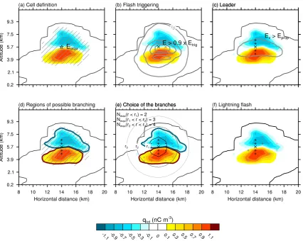
The different steps of the lightning flash scheme are sketched in Fig. 1 and described in this section.

2.2.1 Electrified cells identification

Fig. 1. Different steps of the lightning flash scheme illustrated on a two-dimensional cross section of the total charge density (colored

area; nC m−3). The black line represents the cloud contour. (a) Cell definition: the star locates the grid point where||E||is maximum (Emax). The dashed area delineates the electrified cell. (b) Flash triggering: the grey contours represent||E||with 10, 30, 50 and 70 kV m−1 contours. The crosses show the grid points where||E||> Etrig. The black cross locates the origin of the flash. (c) Bidirectional leader: the

gray contour shows locations whereEz> Eprop. The cross and the + show the grid points where the flash is initiated and where the leader

propagates, respectively. (d) Regions of possible branching: the blue (red) contours limit the regions with negative (positive) total charge density where the negative (positive) branches can propagate. (e) Choice of the branches: the grey points represent the grid points with possible branching between two successive circles (or spheres in 3-D).N ll(r)is the maximum number of branches between two circles of radiusrandr+dr(see Eq. 7). Here, the maximum number of branches is given for a 2-D framework and a mean grid size of 1450 m.

(f) Lightning flash: the resulting lightning flash path made up with the triggering point (black cross), the bidirectional leader (black +) and

the branches (grey +).

area and for a rather short duration time. Therefore, only a few electrified cells were present in the simulation domain at the same time, but the goal now is to treat the individual flashes of several cells simultaneously.

An iterative algorithm is first developed to identify all the electrified cells in the domain of simulation. In the follow-ing, a cell is termed “electrified” if conditions to trigger and to propagate a flash inside it are fulfilled. The elec-tric field module is first multiplied by a factor to get free of the height effect. It is notedE0and corresponds to the electric field module reduced to the ground level. The peak value of E0, Emax, is sought in each subdomain. Then, the global value of the maximum electric field Emaxll=

MAX(Emax)is determined and the processor number (IPcell) whereEmax ll=Emaxis identified. IfEmaxllis higher than 200 kV m−1, the electric field threshold for flash trigger-ing at the ground level (see Sect. 2.2.2), a first electrified cell is detected. The maximum electric field is a natural marker of lightning-triggering cells since a flash is triggered only if Emax>200 kV m−1_{. The point where Emaxll >} 200 kV m−1_{is hereafter called the cell center. The local} co-ordinates of the cell center and IPcellare then broadcast to all processors.

projected onto the horizontal plane of the running level and contiguous grid points are tagged if they meet the following conditions:

– rtot>1×10−5kg kg−1to restrict a flash propagation to a single cloud,

– at least one hydrometeor category has| ˜qx|>q˜cellwhere

˜

qcellis a given threshold to isolate individual storm cells.

˜

qxis the volume charge density (C m−3) for speciesx.

The process is repeated along the horizontal until no more grid points can be added to the cell volume. Updates in the halo zones (in a parallel architecture, a “halo” zone contains the overlapping grid-points which are exchanged with the neighbor processors) are necessary because electrified cells may span over several neighboring subdomains. Then the algorithm loops to analyse the electric field out of the electri-fied cell to find out if another disjuncted electrielectri-fied cell exists in the whole domain.

2.2.2 Flash triggering

The local electric field condition which initiates a flash, fol-lows MacGorman et al. (2001) and Barthe and Pinty (2007b). The triggering electric field,Etrigdecreases with altitude as observed by Marshall et al. (1995):

Etrig= ±167×1.208exp _−z

8.4

(6) wherezis the altitude (km) andEtrigis given in kV m−1. To account crudely for grid scale uncertainty, a flash is triggered where the electric field exceeds a slightly smaller value than Etrig(such ask×Etrig, withk=0.9). If more than one grid point per convective cell meets the conditionE >0.9×Etrig, then the triggering point is chosen at random (Fig. 1b).

The processor IPtrigcontaining this point is identified. The value of the triggering electric field, the coordinates of the flash origin and the sign of the vertical component of the electric field at this point are broadcast from IPtrigto all pro-cessors. This procedure is repeated for each cell. Then, if several cells exist in the domain several flashes can be treated simultaneously since there is a mask that discriminate the dif-ferent cells in the domain.

Once the characteristics (center and extension) of all elec-trified cells are available, the lightning flash stage follows. The treatment of the flashes is broken down into two parts with a “leader” phase that precedes a phase that generates the branches.

2.2.3 Bidirectional leader

The approach follows Helsdon et al. (1992) that relies on the bidirectional leader theory of Kasemir (1960). Kasemir as-sumes that the flash leader propagates bi-directionally from the triggering point, in the parallel and anti-parallel direc-tions of the ambient electric field. The propagation is stopped

once the electric field drops below a threshold value. As previously done by Helsdon et al. (1992), Barthe and Pinty (2007b) simplified this concept since they used the ambient electric field to control the leader propagation instead of the total electric field. They acknowledged that it was a short-coming, but argued that computing the local electric field at the tip of each segment added to the leader was computation-ally expensive. In the present scheme, a new simplification is considered, still for a sake of reducing the computational cost. The bidirectional leader is allowed to propagate along the vertical axis only and not slantwise alongEas in the pre-vious scheme, to avoid communication between the proces-sors each time a new segment is added at the tip of the leader. The two branches of the leader propagate until the ambient vertical electric field (Ez) at the tips of the last segments falls

below∼15 kV m−1_{or when the sign of the vertical} compo-nent of the electric field reverses (Fig. 1c).

As in other studies (MacGorman et al., 2001; Mansell et al., 2002; Barthe et al., 2005; Mansell et al., 2005, 2010), a flash is categorized as “cloud-to-ground” (CG) when the lower end of the leader reaches the bottom of the cell which altitude is below 2 km above ground level (AGL). CG flashes are artificially prolonged to the ground.

Only processor IPcell is in charge of the bidirectional leader. The coordinates of the leader channel and the flash type are broadcast to all processors.

2.2.4 Horizontal extension of the flash

VHF mapping systems have highlighted the extensive hor-izontal structure of lightning flashes in two distinct layers (Shao and Krehbiel, 1996; Rison et al., 1999; Thomas et al., 2001; Wiens et al., 2005; Bruning et al., 2007), with a sin-gle vertical channel connecting the two layers. Therefore, in this context, the new lightning flash scheme must repro-duce this feature but in an economical way, since a phys-ically consistent representation of the discharges is too ex-pensive and would be technically impraticable on powerful massively parallel computers.

According to VHF observations, a positively and a neg-atively charged region must be delineated (propagation is not allowed in a third region in case of a tripole structure of charges). The positively and negatively charged regions where the flash can propagate are explored separately. From the positive part of the leader, the region with negative to-tal charge density where the positive branches can propagate is explored. First, a 3-D mask M(:,:,:)is initialized with value equal to 1 where grid points are reached by the positive leader. Then the neighboring grid points matching the fol-lowing conditions are selected as part of the negative charge pocket:

– the grid point belongs to the electrified cell of the leader

– | ˜qtot|>qcell˜

The fields in the halo zones are updated to allow a contin-uous extension of the pocket of negative charge to nearby subdomains. This step is resumed until no more point can be added. The positive charge pocket is build the same way around the negative leader, leading to two regions of oppo-site charge embedded in the electrified cell contour (blue and red contours in Fig. 1d).

2.2.5 Distribution of the branches

Williams et al. (1985) initiated discharges through plastic slabs with regions of stronger and weaker negative charge density. They observed that the discharges tend to propa-gate toward regions of high charge density, which underlined the importance of the charge density in discharge propaga-tion. Niemeyer et al. (1984) showed that a stochastic dielec-tric breakdown model naturally leads to a fractal structure of the discharge. Tsonis and Elsner (1987) analyzed a set of lightning pictures and deduced an average fractal dimen-sion of the lightning projection. The dielectric breakdown model has been widely used in the past to simulate different types of lightning discharges (Wiesmann and Zeller, 1986; Wiesmann, 1988; Petrov and Petrova, 1993; Sa˜nudo et al., 1995; Kawasaki and Matsuura, 2000, among others). How-ever, none of these studies simulated lightning discharges in a real storm context. Mansell et al. (2002) first introduced the dielectric breakdown concept to simulate the lightning flashes in a cloud model. Then Barthe and Pinty (2007b) de-veloped a probabilistic branching algorithm adapted from the dielectric breakdown concept to mimic the horizontal exten-sion of the flash toward regions of high charge density. The present scheme keeps the idea of charge density criterion to build a 3-D branched discharge (Williams et al., 1985) and to monitor the fractal nature of the flash (Niemeyer et al., 1984) as previously highlighted.

The electrified cell domain is divided into concentric spheres with radius r centered on the triggering point (Fig. 1e). The global number of branchesN llat a distance rfrom the triggering point is assumed to follow a fractal law (Niemeyer et al., 1984):

N ll(i)= Lχ

Lmean

iχ−1 (7)

withLmean, the mean mesh size (m), Lχ, a characteristic

length scale (m), andχ, the fractal dimension (2< χ <3 ac-cording to Petrov and Petrova (1993)). The running integer i, computed asi=NINT(r/Lmean), varies fromimin=0 to imaxwhereimaxcorresponds to the maximum distance where branching is possible, i.e. for gridpoints belonging to mask M. NINT is a function returning the nearest integer of a real number.

So a local array A that contains all the nearest integer dis-tances i between the triggering point and each grid point passing mask M(:,:,:)=1 is filled in each subdomain. The

minimum (imin) and maximum (imax) distances are checked so that the next steps are iterated forimin≤i≤imax.

On each processor, the number of grid points belonging to mask M and located at distancei(Nposs(i)) is computed and summed over all processors to get the global number of possible locationsNposs ll(i). ThenNposs ll(i)is compared toN ll(i)of Eq. (7):

– ifNposs ll(i)≤N ll(i): all the possible grid points at distanceifrom the triggering point are selected, – ifNposs ll(i) > N ll(i): too much grid points are found

so a subset must be selected at random.

In order to randomize properly the selection of the grid points which are dispersed on several subdomains, two 1-D working arrays V(:)and V0_{(:)of sizeNposs ll(i)are allocated}

to each subdomain. Each processor packs the 3-D array A into a 1-D array V under a running mask control defined by A(:,:,:)=i. V0is initially set to 0.

The number of grid points,Nposs(i), at a given distancei is gathered by each processor and the result is broadcast to all processors. Consequently, each of the IPflash processor knows the proportion of grid points which is granted in its physical subdomain since the total lightning flash path should contain at mostN ll(i)grid points. A random integernis then taken in the interval 0 andNposs ll(i). The grid point number V(n)is extracted and element V0(V(n))is turned to 1. This step is repeated untilN ll(i)points are chosen. Fi-nally, the elements ofV0are scattered (equivalent to an un-pack operation) in a 3-D array S(:,:,:)under the same mask condition A(:,:,:)=i. As a result, the sparse array S(:,:,:) obtained at the last iterationi=imax, marks the full path of the lightning flash (Fig. 1f). The branches coordinates are then broadcast to all processors.

Compared to the original scheme of Barthe et al. (2005), the new lightning scheme ignores deliberately any rules of connectivity that should apply to the grid points tracing the flash path. The higher randomization and consequently the lack of structuration of the branching phase is the price to pay to get a parallel source code even if it is done essentially for technical reasons. We believe however that running sim-ulations of electrified storms on large grid systems, and so accessing to parallel computing, is very promising for real meteorological applications of cloud electricity.

2.2.6 Neutralization

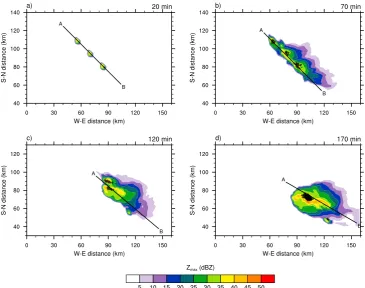
Fig. 2. STERAO storm: Simulated composite radar reflectivity (Zmax, in dBZ) at (a) 20 min, (b) 70 min, (c) 120 min and (d) 170 min. The

+ symbols indicate the origin of the lightning flashes in a 10-min interval from the time of the cross section. The black line segment [AB] corresponds to the location of the vertical cross sections of Fig. 3.

Once the charge is neutralized, the electric field is updated. If at least one new triggering point is found in the domain, the procedure (from Sect. 2.2.3 to Sect. 2.2.6) is repeated. Thus, in a single time step, each cell can generate several flashes. 2.3 Technical aspects

The whole scheme is embedded in the cloud-resolving meso-cale model Meso-NH in which the resolved-smeso-cale and turbu-lent transport terms (Eqs. 1 and 3) are computed. The code is written in Fortran 90 and parallelization is obtained by using MPI functions. The bulk electrical charge scheme is developped in the framework of the single moment micro-physical scheme of Meso-NH to take advantage of calculat-ing the mass microphysical rates (to get the transfer ratesTxq

in Eq. 1). The inversion of Eq. (5) to extractV0 is done by direct and inverse FFT on the horizontal and by resolving a tridiagonal system along the vertical. The computation ofE is exact in absence of orography. In the other case (orogra-phy is present), a conjugate gradient method or equivalent which implies an iterative loop, is necessary to include cross derivative terms. The lightning flash scheme excepted, the computation of the charges and of the electric field are not easily adaptable to other models.

CELLS v1.0 is then available in the release of Meso-NH v4.9. The use of the Meso-NH model by groups other than the developers is subject to a licence agreement. Additional details on the Meso-NH model appear in http://mesonh.aero. obs-mip.fr/mesonh/ with technical and scientific documenta-tion.

3 Simulation of the lightning activity during the 10 July 1996 STERAO storm

Fig. 3. STERAO storm: Vertical cross sections of the total charge density (colors; in nC m−3) along the [AB] segment defined in Fig. 2 at

(a) 20 min, (b) 70 min, (c) 120 min and (d) 170 min. The black solid line corresponds to the cloud contour. Dashed gray contours show the

electric field module (10 and 50 kV m−1contours).

3.1 Numerical set-up

The numerical simulation was performed with the non-hydrostatic mesoscale model Meso-NH version 4.8.4. The environment was assumed to be homogeneous, then a single profile was used for initialization (Skamarock et al., 2000). As in previous numerical studies of this storm (Skamarock et al., 2000, 2003; Barth et al., 2001, 2007; Barthe et al., 2007; Barthe and Barth, 2008), three warm bubbles (+3◦C) were oriented in a north-west to south-east line (Fig. 2a). A 160×160 km2horizontal domain was used with a 1-km res-olution. The vertical grid had 51 levels up to 23 km with a level spacing of 50 m close to the surface stretching to 700 m at the top of the domain. The time step was 2.5 s, and the simulation lasted 3 h.

The physics of the model included a mixed-phase micro-physics scheme (Pinty and Jabouille, 1998) and a 3-D tur-bulence scheme (Cuxart et al., 2000). The parameterization of Takahashi (1978) is used to describe the NI processes as in the previous simulation of this storm by Barthe et al. (2007). To prevent unreasonably large charging and flash rates, the magnitude of charge separated per rebounding col-lision is limited to 100 fC, 30 fC and 10 fC for snow-graupel,

ice crystal-graupel and ice crystal-snow collisions, respec-tively. The branching parametersχandLχare set to 2.3 and

1500 m, respectively. The impact of these parameters on the flash rate and lightning characteristics will be investigated in Sect. 3.4.

3.2 Dynamics, microphysics and charge structure

The transition occurred after 150 min of simulation while Skamarock et al. (2000) estimated the real system transi-tionned after 3 h of active convection so the model is fairly successful in reproducing the evolution of the storm.

Vertical cross sections of the total charge density along the wind axis at 5 km altitude were performed at different stages of the storm to analyze the charge structure and its evolu-tion. At 20 min (Fig. 3a), the south-eastern cell was the first one to become electrified. Charges were separated by the non-inductive mechanism at∼7.5 km altitude, generating a negative dipole (negative charge layer above positive charge layer) centered at 7.5 km altitude above sea level (ASL). As a result, the electric field increased above 10 kV m−1at the interface of the two layers of opposite charge. 50 min later (Fig. 3b), the total charge density exhibited a more complex structure, alternating between tripoles in the convective cores and positive dipoles in the cloud anvils. A negative screen-ing layer due to negative ions was visible at the top of the cloud. At 120 min (Fig. 3c), during the transition stage, the charge structure looked like a tripole. Positively charged ice crystals were responsible for the upper positive charge layer, while snow and graupel particles were involved in the main negative layer. The positive charge layer above the ground was made up with positive graupel which fell below the 0◦C isotherm and melted into positive raindrops. During the su-percell stage (170 min; Fig. 3d), the charge structure evolved between a dipole and a tripole, depending on the location in the storm. Negative ice crystals were advected in the anvil (not shown).

3.3 Lightning characteristics

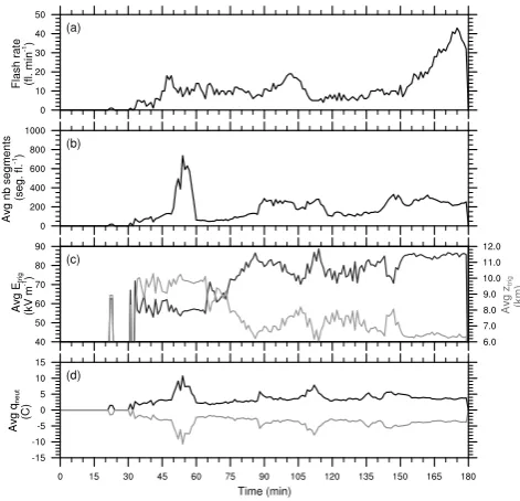
The flash rate is displayed in Fig. 4a for the 3 h of simula-tion. During the multicell stage, the flash rate does not ex-ceed 20 fl. min−1which is significantly lower than the obser-vations. Defer et al. (2001) reported indeed a maximum of 50 fl. min−1 at∼23:45 UTC from the ONERA (Office Na-tional d’Etudes et Recherches A´erospatiales) VHF interfer-ometric mapper (ITF). However, during the multicell stage, a large portion of the flashes detected by the ITF were iden-tified as duration” flashes. At 23:30 UTC, the “short-duration” flash ratio per 5-min period raised up to 0.46 (as estimated from Fig. 10 of Defer et al., 2001). The simulated flash rate decreases at 110 min, and reaches a plateau (∼5– 10 fl. min−1) until 150 min. The flash rate detected by the ITF (∼10–35 fl. min−1_{) is still larger than the simulated one.} During this stage of the storm, the “short-duration” flash ratio reaches 0.2. Then, the flash rate increases up to 44 fl. min−1 during the supercell stage, while in the observations, it peaks at 45 fl. min−1.

Figure 4b–d shows the 1-min averaged number of seg-ments, triggering altitude, triggering electric field and pos-itive and negative charge neutralized. One can note that the average number of segments is less than 400 segments per flash except a peak of 700 segments per flash during the

Fig. 4. STERAO storm: Time evolution of (a) the flash rate (fl. min−1), (b) the average number of segments per flash, (c) the average triggering electric field (black curve; kV m−1) and trigger-ing altitude (gray curve ; km), and (d) the average positive (black curve) and negative (gray curve) charge neutralized per flash (C). The number of segments, the triggering electric field, the trigger-ing altitude and the charge neutralized are averaged over a 1-min interval.

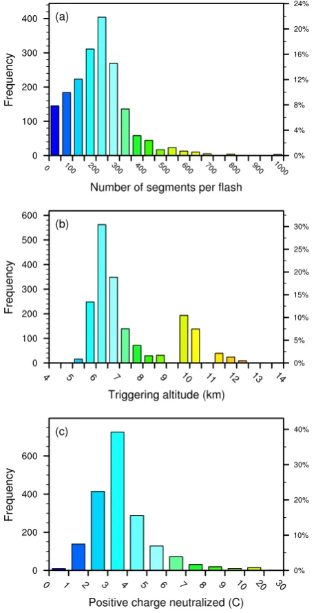
multicell stage (Fig. 4b). The histogram showing the num-ber of segments per flash confirms that 91 % of the flashes have less than 400 segments (Fig. 5a).

In the first part of the multicell stage (30–60 min), the av-erage triggering altitude is 10 km a.s.l., then it decreases to 6–8 km altitude (Fig. 4c). Figure 5b confirms that two differ-ent layers exist for flash triggering. Most of the flashes are triggered between 5.5 and 7 km a.s.l., between the main neg-ative charge and the lower positive charge (Fig. 3). Note that the triggering altitude and the triggering electric field have an opposite evolution (Fig. 4c) as expected from Eq. (6).

The total electric charge neutralized per flash lays between 0.4 and 20.23 C. The temporal evolution of the 1-min aver-aged neutralized charge shows that a peak occurs between 45 and 60 min which is associated with the larger number of segments. More than 60 % of the flashes neutralize be-tween 1 and 4 C. These results are in agreement with data reported in the literature. Indeed, from modeling studies, the charge transfer during intra-cloud discharges was estimated to be between∼2.7 C and∼52.4 C (MacGorman et al., 2001; Mansell et al., 2002; Riousset et al., 2007). Similar values were found from observational studies (Krehbiel, 1981; Shao and Krehbiel, 1996; Rakov and Uman, 2003).

Fig. 5. STERAO storm: Histograms of (a) the number of segments

per flash, (b) the triggering altitude (kV m−1) per flash, and (c) the charge neutralized (C) per flash. Since all flashes were IC flashes, the same amount of negative charges was neutralized.

Bull Novascale R422 with 20 compute nodes each with 2×2 Intel Xeon processors quadcore 2.26 Ghz and 24 GB of mem-ory). About 30 % of the computing time is attributed to the electrical scheme for this simulation on 16 processors. 3.4 Sensitivity analysis

Since the electrical scheme results rely on several thresholds (for charge separation, cell detection, branching and charge neutralization), it is important to investigate the impact of varying the value of these thresholds.

3.4.1 Non-inductive parameterization

Several studies (Helsdon et al., 2001; Mansell et al., 2005; Altaratz et al., 2005; Barthe and Pinty, 2007a) have investi-gated the sensitivity of the flash rate to the NI parameteriza-tion which is recognized as the process mainly responsible for charge separation (Reynolds et al., 1957; Williams and Lhermitte, 1983; Dye et al., 1989; Latham et al., 2007). To prevent unreasonably large charging and flash rates, the mag-nitude of the charge exchanged per rebounding collision (δq) is generally limited. Mansell (2000) limitedδqto 200 fC for graupel-snow collisions and 2 fC for graupel-crystal interac-tions. Mansell et al. (2005) revised theseδq values to 50 fC and 20 fC for rebounding graupel-snow and graupel-crystal collisions, respectively.

Increasing δq leads to an increase of the number of flashes as shown in Table 1. With the recommended set-ting of Mansell et al. (2005) (NI1 case), 752 flashes are triggered, while if the charge exchanged per collision is un-bounded (NI3 case), 10 times more flashes are produced (7534 flashes). The NI2 case is intermediate between NI1 and NI3. From NI1 to NI3, the number of segments is in-creased by a factor 3 leading to a higher quantity of charge neutralized per flash (2.98 C vs. 4.36 C on average). Conse-quently, the total charge neutralized during the storm is∼14 times higher in the NI3 test (32813.6 C) than in the NI1 test (2242.5 C). Note that the first flash in NI3 is triggered 13 min before the first flash in NI1 as a result of allowing a larger charging rate. The flash rate evolution keeps the same trend whatever the peak valueδq is set to.

The structure of the total charge density does not depart from the tripole (Fig. 3) when the limitation of the amount of neutralized charge per rebounding collision is changed (not shown). The total charge density never exceeds±3 nC m−3 and||E||remains under 110 kV m−1 for the NI1, NI2 and NI3 cases. If the charge exchanged per collision is unlim-ited, the maximum charging rate is 288 pC m−3s−1for snow-graupel interactions and never exceeds 130 pC m−3s−1 for ice crystal-snow and ice crystal-graupel elastic collisions.

In conclusion, even if the flash rate is sensitive to the set-ting ofδq, the charge structure which depends on the tem-perature and on the microphysical composition (NI charg-ing processes) is not impacted. Moreover, the new lightncharg-ing scheme is efficient to limit the total charge density and the electric field module to acceptable values. In the following, the NI2 setting of the NI charging parameters which leads to the best flash data comparison with Defer et al. (2001), is preferred.

3.4.2 Lightning scheme parameters

Table 1. Summary of the sensitivity tests related to the limitation of the quantity of charge separated per rebounding collision.

δq_SGmax/δq_IGmax/δq_ISmax Number 1st flash Number Triggering Etrig Mean charge Total charge

(fC) of flashes (s) of segments altitude (km) (kV m−1) per flash (C) neutral. (C) NI1 50/20/2 752 2027.5 111±62 8.33±1.82 68.6±15.1 2.98±1.11 2242.501

Mansell et al. (2005) [18–317] [5.44–12.40] [41.3–95.2] [0.77–8.21]

NI2 100/30/10 1849 1367.5 212±122 7.33±1.65 77.2±13.6 3.72±1.57 6880.18 Present Study [6–997] [5.09–13.10] [37.9–98.6] [0.40–15.11]

NI3 all at 1.1015 7534 1220.0 340±266 6.91±1.34 81.9±11.2 4.36±2.06 32813.61 No Limitation [9–2249] [4.46–14.50] [33.0–109.2] [0.26–20.23]

charge neutralization valueq˜neut. Results are reported in Ta-ble 2.

When the threshold for cell detectionqcell˜ is decreased in Q1, the size of the detected cells is larger. At the begining of the simulation when the three cells are well separated, this re-sults in few differences. However after 30 min of simulation when the cells start to merge, the cell detection algorithm recognizes a single “big cell”. Consequently, the lightning flashes are allowed to spread horizontally over the artificially “big cell”, while the three original cells are still distinguish-able. Decreasing q˜cell leads to slightly less flashes (1727 vs. 1849), but with a significantly wider extension (438 vs. 212 segments) and charge neutralization efficiency (4.32 C vs. 3.72 C).

If the charge neutralization thresholdq˜neutis increased to 0.2 nC m−3in Q2, it is expected that the charge neutralized per flash decreases as well (2.06 C vs. 3.72 C). As a conse-quence, the number of flashes is increased (3361 vs. 1849) but a similar total charge amount is neutralized (6933.74 C vs. 6880.18 C). Note that for all the experiments reported in Table 2, the mean triggering altitude lies between 7.21 km and 7.39 km, except for simulation Q2 where it is higher (8.68 km). This increase of the mean triggering altitude is due to a larger proportion of flash triggered between the up-per positive and the middle negative charge layers in Q2 com-pared to REF. In Q2, more than 50 % of the flashes are trig-gered between 10 and 12 km altitude, while this proportion falls down to 20 % in REF (not shown). A possible expla-nation for this difference can be found in Figs 3b and 3c. The total charge density has a higher value in the lower pos-itive charge layer (0.1–1 nC m−3) than in the upper positive charge layer (0.1–0.5 nC m−3). Then, if the charge neutral-ization threshold is increased, the flashes triggered in the up-per part of the cloud will neutralize less charges than the ones initiated in the lower part of the cloud. So because they are less efficient, more flashes are needed to neutralize the same amount of charge in the 10–12 km layer.

In agreement with Barthe and Pinty (2007b), ifχ is in-creased, the number of flashes decreases while the number of segments per flash (given by Eq. 7) and consequently, the amount of neutralized charge per flash increases. Keeping

identical the NI parameterization andδq in the C1-C4 sim-ulations, the total charge neutralized differs by only 13.5 % between C1 (χ=2.1) and C4 (χ=2.9). Whenχis held con-stant (χ=2.3) andLχis increased from 500 m to 2500 m in

L1–L2, the average number of segments per flash increases by a factor 3.4. As a consequence, the mean neutralized charge is higher forLχ=500 m than forLχ=2500 m by

a factor 2.5. The L1 simulation is the only one that pro-duces CG flashes for the STERAO storm. All are negative CGs. The first CG is produced at 94 min, and the three others are triggered between 157 and 159 min. The main difference with the other simulations lies in the relatively low number of segments per flash in L1 (91.1±60.5), leading to a lower average neutralized charge per flash (2.01±1.11 C).

Table 2. Summary of the sensitivity tests related to the flash propagation. In all these simulations, the first flash occurrence is 1367.5 s.

˜

qcell qneut˜ χ Lχ Number Number Triggering Mean charge Total charge

(nC m−3) (nC m−3) (m) of flashes of segments altitude(km) per flash (C) neutral. (C) REF 0.2 0.1 2.3 1500 1849 212±122 7.33±1.65 3.72±1.57 6880.18

0 CG [6–997] [5.09–13.10] [0.40–15.11]

C1 0.2 0.1 2.1 1500 2113 156.9±86.8 7.35±1.67 3.15±1.28 6651.77 0 CG [12–738] [5.09–13.10] [0.74–12.17]

C2 0.2 0.1 2.5 1500 1681 281.2±154.6 7.34±1.65 4.28±1.93 7197.87 0 CG [16–1089] [5.44–13.1] [0.94–20.77]

C3 0.2 0.1 2.7 1500 1484 369.5±204.8 7.30±1.64 5.01±2.22 7430.53 0 CG [16–1204] [5.09–13.1] [1.33–21.93]

C4 0.2 0.1 2.9 1500 1325 463.0±254.7 7.31±1.63 5.75±2.61 7612.79 0 CG [19–1241] [5.09–13.1] [1.38–22.32]

L1 0.2 0.1 2.3 500 3156 91.1±60.5 7.39±1.65 2.01±1.11 6357.53

−2.01±1.01 −6330.40 4 CG [8–642] [5.09–13.1] [0.10–24.45]

[−12.22—0.10]

L2 0.2 0.1 2.3 2500 1415 305.7±158.6 7.29±1.63 5.04±2.06 7127.98 0 CG [19–951] [5.09–12.4] [1.44–22.27]

Q1 0.1 0.1 2.3 1500 1727 438.2±241.5 7.21±1.60 4.32±2.22 7462.54 0 CG [17–1147] [5.09–13.80] [0.96–34.42]

Q2 0.2 0.2 2.3 1500 3361 274.7±208.9 8.68±2.16 2.06±1.69 6933.74 0 CG [5–1330] [5.09–13.80] [0–13.82]

4 The 21 July 1998 EULINOX storm case

The 21 July 1998 EULINOX (European Lightning Nitrogen Oxides Project) storm case (Huntrieser et al., 2002) is sim-ulated to evaluate the tuning of the new lightning flash pa-rameters for a severe event that developped on the evening, West of Munich, Germany. After a first period of intensi-fication, the storm split into two distinct cells. The north-ernmost cell became multicellular in structure and was ob-served to decay soon after the cell-splitting event, while the southern cell strengthened and developed supercell charac-teristics. Cloud-to-ground discharges were recorded by an LPATS (Lightning Position and Tracking System) system, while the total lightning activity (IC + CG) was mapped by the ONERA interferometer. This storm has been previously simulated with the Penn State/NCAR Mesoscale Model 5 (MM5) (Fehr et al., 2004) and the 3-D Goddard Cumulus Ensemble (GCE) Model (Ott et al., 2007) to investigate light-ning NOxproduction and transport.

4.1 Numerical set-up

The simulation performed is similar to Fehr et al. (2004). A single thermodynamic composite sounding is used to ini-tialize the storm (see Fig. 4 in Fehr et al., 2004). The con-vection is initiated with a warm (3◦C perturbation) bubble.

The model domain is chosen to be 180×180×23 km3 in x,y, andzdirections with 1 km horizontal grid spacing and 51 grid points in the vertical direction, with a variable res-olution beginning at 250 m at the surface and stretching to 500 m at the top of the domain. The simulation is integrated with a 2.5 s time step for a 3 h period.

As in the 10 July 1998 STERAO simulation, the physics of the model included a mixed-phase microphysics scheme (Pinty and Jabouille, 1998) and a 3-D turbulence scheme (Cuxart et al., 2000). The parameterization of Takahashi (1978) is used to describe the non-inductive processes. The lightning scheme parameters are the same as for the STERAO storm simulation. The maximum magnitude of charge separated per rebounding collision is limited to 100 fC, 30 fC and 10 fC for snow-graupel, ice crystal-graupel and ice crystal-snow collisions, respectively. The branching parametersχandLχare set to 2.3 and 1500 m, respectively.

4.2 Results: electrical activity

Fig. 6. EULINOX storm: (a/c) Simulated composite radar reflectivity (Zmax, in dBZ) and (b/d) vertical cross section of the total charge

density (colors ; in nC m−3) along the [AB] segment defined in (a/c) at 60/120 min. The + symbols indicate the origin of the lightning flashes in a 10-min interval from the time of the cross section.

Fig. 7. EULINOX storm: Lightning flash characteristics as simulated by Meso-NH with (a) temporal evolution of the total (black curve) and

turned into a multicell and remained in the domain for the rest of the simulation.

The electrical structure is shown in Fig. 6b and 6d. At 60 min, the storm shows a forward tilted tripole, except for the anvil with a slightly positive dipole. The highest charges are found in the updraft core at 5–6 km altitude. At 120 min, the updraft charge structure of the southern cell is much complex and an inverted dipole tends to emerge in the anvil (Fig. 6b and d).

The flash rate simulated by Meso-NH for the 21 July 1998 EULINOX storm is shown in Fig. 7. The first flash is trig-gered after 19 min of simulation. Then, during 75 min, the total flash rate ranges between 5 and 15 fl. min−1. This corre-sponds to the first stage of weak lightning activity observed and reported by Fehr et al. (2004) (see their Fig. 6b) with a slow increase of the total flash rate close to 10 fl. min−1. After 75 min, the flash rate increases and reaches a peak of 58 fl. min−1_{at 128 min. Then, the flash rate remains in the} range 35–55 fl. min−1 _{until the end of the simulation. This} sequence is slightly different in the observations. First the total lightning activity achieved an abrupt increase up, to 52 fl. min−1 around 17:45 UTC, i.e. ∼95 min after the first flash was detected by the ITF. Then, the observed total flash rate decreased gradually until 19:00 UTC (∼20 fl. min−1). At this time however, Fehr et al. (2004) indicated that the lightning flash detection efficiency was possibly degraded when the supercell moved over the interferometer antenna. Meso-NH produced 4521 flashes, 33 of them being cloud-to-ground flashes, representing 0.7 % of the total lightning activity. Fehr et al. (2004) reported that 3321 flashes were detected, and 7 % were cloud-to-ground flashes. So one can estimate that Meso-NH is able to reproduce the character-ics (amplitude and time evolution of the total flash rate) of the EULINOX storm approximately but the cloud-to-ground proportion is clearly underpredicted by a factor 10. This is not surprising since the criterion to decide the formation of cloud-to ground flashes must be refined.

The histograms of the number of segments per flash (Fig. 7b) shows that almost 85 % of the lightning flashes are made up of less than 600 segments, the average number of segments per flash being 348 segments per flash. As in the STERAO storm, lightning flashes are preferentially triggered in two layers (Fig. 7c): 5.5–6.5 km and 10–12 km, which is consistent with the charge structure displayed in Fig. 6b and 6d. Each flash neutralizes 5.02 C on average.

In conclusion, Meso-NH succeeded in reproducing the EULINOX storm and its lightning activity in case of highly simplified environmental conditions. This is a first step since only a full real case simulation followed by a direct compari-son with detailed lightning measurements (Ricompari-son et al., 1999) allows an unambiguous validation of the electrical scheme.

For the EULINOX simulation performed on 32 processors of the CCUR, the electrical scheme computation represents 40 % of the total computing time. The computing time due

to CELLS is expected to vary with more or less lightning activity in the domain.

5 Conclusions

In this paper, we report the recent improvements brought to the electrification and lightning flash scheme in Meso-NH. The governing equations of the electric charge carried by the condensed species (including hail) are completed by two equations treating the physics of positive and negative ions. Ions ensure a continuity of the electric charge out of the clouds and the precipitation in particular when particules evaporate. The ions are also responsible of the screen charge layers which form on the edge of electrified clouds.

The most important change however concerns the light-ning flash scheme which has been heavily revised in order to be run in a multi-processor environment. The treatment of the flashes is the bottleneck of an electrification scheme because the filamentary aspect of the channel which needs to be resolved at high resolution, imposes to develop an algo-rithm which is not suitable to parallelization. Previously, the growth of the lightning discharge was based on a recursive description of the flash propagation into positive and negative pockets of charges. Here recursion comes from the rule that at a given stage of the flash, new segments are added only after a random selection of all the possible grid points that can be connected to the current structure. The new scheme simplifies this view by relaxing the connectivity criterion in order to select at once all the grid points of the flash structure. The new flash algorithm identifies first all the indepen-dent electrified cells in order to prepare a parallel treatment of all flashes that propagate inside the cells. In most of the cases, an electrified cell is split over several subdomains on a distributed-memory computer. A bidirectional leader phase of the flash is defined for each cell with an upward and down-ward vertical tracing from the flash triggering grid point. The density of the branches is assumed to follow a fractal law so that the number of grid points reached by the flash increases with the distance from the triggering point. These distances, filtered by an electric charge density conditions, are com-puted by the processors attached to the subdomains where the flash propagates and the corresponding end grid points are stored. Then a subset of grid points at an equal distance from the triggering point are selected at random in order to fit the number of points deduced by the fractal law for this distance. All these operations can be parallelized owing an exchange of messages between all processors.

favorably the thousands of flashes in both cases but with a few number of CG flashes, obtained for the EULINOX case only. A sensitivity study carried out for the STERAO case helped to limit some excessive NI charging rates and to esti-mate non-measurable flash parameters.

The next step is to run the electrical scheme for storms developing over complex terrain in order to verify that the new lightning scheme supports well a high coordinate dis-tortion as anticipated. This objective is part of the HyMeX experiment planned in 2012 with the purpose of studying the heavy rainfalls produced by electrified orographically-forced storms in the South of France.

Acknowledgements. Computations have been performed on the

supercomputer facilities of Universit´e de la R´eunion and on the 30 node home-made cluster of Lab. A´erologie (2.4 GHz ”Xeon Ne-halem” QuadCore biprocessor per node and 40 Gb/s ”InfiniBand” interconnect network). J-P Pinty acknowledges CICT (Centre Interuniversitaire de Calcul de Toulouse) of University of Toulouse for access to supercomputer “hyperion” where useful simulations could be done additionally.

Edited by: V. Grewe

References

Altaratz, O., Reisin, T., and Levin, Z.: Simulation of the elec-trification of winter thunderclouds using the three-dimensional Regional Atmospheric Modeling System (RAMS) model: Sin-gle cloud simulations, J. Geophys. Res., 110, D20205, doi:10.1029/2004JD005616, 2005.

Avila, E. E., Varela, G. G. A., and Caranti, G. M.: Temperature de-pendance of static charging in ice growing by riming, J. Atmos. Sci., 52, 4515–4520, 1995.

Barth, M. C., Stuart, A. L., and Skamarock, W. C.: Numerical sim-ulations of the July 10, 1996, Stratospheric-Tropospheric Exper-iment: Radiation, Aerosols, and Ozone STERAO- Deep con-vection experiment storm: Redistribution of soluble tracers, J. Geophys. Res., 106, 12381–12400, doi:10.1029/2001JD900139, 2001.

Barth, M. C., Kim, S.-W., Wang, C., Pickering, K. E., Ott, L. E., Stenchikov, G., Leriche, M., Cautenet, S., Pinty, J.-P., Barthe, Ch., Mari, C., Helsdon, J. H., Farley, R. D., Fridlind, A. M., Ack-erman, A. S., Spiridonov, V., and Telenta, B.: Cloud-scale model intercomparison of chemical constituent transport in deep con-vection, Atmos. Chem. Phys., 7, 4709–4731, doi:10.5194/acp-7-4709-2007, 2007.

Barthe, C. and Barth, M. C.: Evaluation of a new lightning-produced NOxparameterization for cloud resolving models and

its associated uncertainties, Atmos. Chem. Phys., 8, 4691–4710, doi:10.5194/acp-8-4691-2008, 2008.

Barthe, C. and Pinty, J.-P.: Simulation of electrified storms with comparison of the charge structure and lightning efficiency, J. Geophys. Res., 112, D19204, doi:10.1029/2006JD008241, 2007a.

Barthe, C. and Pinty, J.-P.: Simulation of a supercellular storm using a three-dimensional mesoscale model with an explicit

lightning flash scheme, J. Geophys. Res., 112, D06210, doi:10.1029/2006JD007484, 2007b.

Barthe, C., Molini´e, G., and Pinty, J.-P.: Description and first results of an explicit electrical scheme in a 3D cloud resolving model, Atmos. Res., 76, 95–113, 2005.

Barthe, C., Pinty, J.-P., and Mari, C.: Lightning-produced NOxin

an explicit electrical scheme: a STERAO case study, J. Geophys. Res., 112, D04302, doi:10.1029/2006JD007402, 2007.

Barthe, C., Deierling, W., and Barth, M. C.: Estimation of total lightning from various storm parameters: A cloud-resolving model study, J. Geophys. Res., 115, D24202, doi:10.1029/2010JD014405, 2010.

Blyth, A. M., Jr., H. J. C., Driscoll, K., Gadian, A. M., and Latham, J.: Determination of ice precipitation rates and thunderstorm anvil ice contents from satellite observations of lightning, Atmos. Res., 59–60, 217–229, 2001.

Bruning, E. C., Rust, W. D., Schuur, T. J., MacGorman, D. R., Kre-hbiel, P. R., and Rison, W.: Electrical and polarimetric radar ob-servations of a multicell storm in TELEX, Mon. Weather Rev., 135, 2525–2544, 2007.

Cecil, D. J. and Zipser, E. J.: Relationships between tropical cy-clone intensity and satellite-based indicators of inner core con-vection: 85-GHz ice-scattering signature and lightning, Mon. Weather Rev., 127, 103–123, 1999.

Chiu, C.-S.: Numerical study of cloud electrification in a axisym-metric, time-dependant cloud model, J. Geophys. Res., 83, 5025– 5049, 1978.

Cuxart, J., Bougeault, P., and Redelsperger, J.-L.: A turbulence scheme for mesoscale and large-eddy simulations, Quart. J. Roy. Meteor. Soc., 126, 1–30, 2000.

Darden, C. B., Nadler, D. J., Carcione, B. C., Blakeslee, R. J., Stano, G. T., and Buechler, D. E.: Utilizing total lightning informa-tion to diagnose convective trends, Bull. Am. Meteorol. Soc., 91, 167–175, doi:10.1175/2009BAMS2808.1, 2010.

Defer, E., Blanchet, P., Th´ery, C., Laroche, P., Dye, J. E., Venticinque, M., and Cummins, K. L.: Lightning activ-ity for the July 10, 1996, storm during the Stratosphere-Troposphere Experiment: Radiation, Aerosol, and Ozone-A (STERAO-A) experiment, J. Geophys. Res., 106, 10151–10172, doi:10.1029/2000JD900849, 2001.

Defer, E., Laroche, P., Dye, J. E., and Skamarock, W. C.: Use of total lightning lengths to estimate NOxproduction in a Colorado

thunderstorm, in: Proceedings of the 12th International Confer-ence on Atmospheric Electricity, 9–13 June 2003, Int. Comm. on Atmos. Electr., Versailles, France, 2003.

Deierling, W., Petersen, W. A., Latham, J., Ellis, S., and Chris-tian, H. J.: The relationship between lightning activity and ice fluxes in thunderstorms, J. Geophys. Res., 113, D15210, doi:10.1029/2007JD009700, 2008.

Dye, J. E., Jones, J. J., and Winn, W. P.: Observations within two re-gions of charge during initial thunderstorm electrification, Quart. J. Roy. Meteor. Soc., 114, 1271–1290, 1989.

experi-ment with results for the July 10, 1996 storm, J. Geophys. Res., 105, 10023–10045, doi:10.1029/1999JD901116, 2000.

Emersic, C., Heinselman, P. L., MacGorman, D. R., and Brun-ing, E. C.: Lightning activity in a hail-producing storm observed with phased-array radar, Mon. Weather Rev., 139, 1809–1825, doi:10.1175/2010MWR3574.1, 2011.

Fehr, T., H¨oller, H., and Huntrieser, H.: Model study on production and transport of lightning-produced NOx in a

EULINOX supercell storm, J. Geophys. Res., 109, 1–17, doi:10.1029/2003JD003935, 2004.

Fierro, A. O., Leslie, L., Mansell, E., Straka, J., MacGorman, D., and Ziegler, C.: A high-resolution simulation of microphysics and electrification in an idealized hurricane-like vortex, Meteor. Atmos. Phys., 98, 13–33, 2007.

Gardiner, B. A., Lamb, D., Pitter, R., Hallett, J., and Saunders, C.: Measurements of initial potential gradient and particle charge in a Montana summer thunderstorm, J. Geophys. Res., 90, 6079– 6086, 1985.

Goodman, S. J., Buechler, D. E., Wright, P. D., and Rust, W. D.: Lightning and precipitation history of a microburst-producing storm, Geophys. Res. Lett., 15, 1185–1188, doi:10.1029/GL015i011p01185, 1988.

Helsdon, J. H. and Farley, R. D.: A numerical modeling study of a Montana thunderstorm: Part 2 : Model results versus obser-vations involving electrical aspects, J. Geophys. Res., 92, 5661– 5675, 1987.

Helsdon, J. H., Wu, G., and Farley, R. D.: An intracloud light-ning parameterization scheme for a storm electrification model, J. Geophys. Res., 97, 5865–5884, 1992.

Helsdon, J. H., Wojcik, W. A., and Farley, R. D.: An examination of thunderstorm-charging mechanism using a two-dimensional storm electrification model, J. Geophys. Res., 106, 1165–1192, doi:10.1029/2000JD900532, 2001.

Helsdon, J. H., Gattaleeradapan, S., Farley, R. D., and Waits, C. C.: An examination of the convective charging hypothesis : Charge structure, electric fields, and Maxwell currents, J. Geophys. Res., 107, 4630, doi:10.1029/2001JD001495, 2002.

Hou, T., Lei, H., and Hu, Z.: Numerical simulation of the re-lationship between electrification and microphysics in the pre-lightning stage of thunderstorms, Atmos. Res., 91, 281–291, doi:10.1016/j.atmosres.2008.04.009, 2009.

Huntrieser, H., Feigl, C., Schlager, H., Schroder, F., Gerbig, C., van Velthoven, P., Flatoy, F., Th´ery, C., Petzold, A., H¨oller, H., and Anann, U.: Airborne measurements of NOx, tracer

species and small particles during the Europeean Lightning Nitrogen Oxides Experiment, J. Geophys. Res., 107, D11, doi:10.1029/2000JD000209, 2002.

Jabouille, P., Guivarch, R., Kloos, P., Gazen, D., Gicquel, N., Gi-raud, L., Asencio, N., Ducrocq, V., Escobar, J., Redelsperger, J.-L., Stein, J., and Pinty, J.-P.: Parallelization of the French Meteorological Mesoscale Model M´esoNH, in: Proceedings of the 5th International Euro-Par Conference on Parallel Process-ing, Euro-Par ’99, 1417–1422, Springer-Verlag, London, UK, UK, available at: http://portal.acm.org/citation.cfm?id=646664. 701041, 1999.

Jayaratne, R., Saunders, C. P. R., and Hallet, J.: Laboratory studies of the charging of soft hail during ice crystal interactions, Quart. J. Roy. Meteor. Soc., 103, 609–630, 1983.

Kajikawa, M. and Heymsfield, A. J.: Aggregation of ice crystals in

cirrus, J. Atmos. Sci., 46, 3108–3121, 1989.

Kasemir, H. W.: A contribution to the electrostatic theory of a light-ning discharge, J. Geophys. Res., 65, 1873–1878, 1960. Kawasaki, Z. and Matsuura, K.: Does a lightning channel show a

fractal?, Appl. Energy, 67, 147–158, 2000.

Keith, W. D. and Saunders, C. P. R.: Further laboratory studies of the charging of graupel during ice crystal interactions, Atmos. Res., 25, 4345–4464, 1990.

Krehbiel, P. R.: An analysis of the electric field change produced by lightning, Ph.D. thesis, Univ. of Manchester Inst. of Sci. and Technol., Manchester, UK, 1981.

Kuhlman, K. M., Ziegler, C. L., Mansell, E. R., MacGorman, D. R., and Straka, J. M.: Numerically simulated electrification and lightning of the 29 June 2000 STEPS supercell storm, Mon. Weather Rev., 134, 2734–2757, 2006.

Lafore, J. P., Stein, J., Asencio, N., Bougeault, P., Ducrocq, V., Duron, J., Fischer, C., H´ereil, P., Mascart, P., Masson, V., Pinty, J. P., Redelsperger, J. L., Richard, E., and Vil`a-Guerau de Arel-lano, J.: The Meso-NH Atmospheric Simulation System. Part I: adiabatic formulation and control simulations, Ann. Geophys., 16, 90–109, doi:10.1007/s00585-997-0090-6, 1998.

Latham, J., Petersen, W. A., Deierling, W., and Christian, H. J.: Field identification of a unique globally dominant mechanism of thunderstorm electrification, Quart. J. Roy. Meteor. Soc., 133, 1453–1457, 2007.

MacGorman, D. R. and Rust, W. D.: The electrical nature of storms, Oxford Univ. Press, 1998.

MacGorman, D. R., Straka, J. M., and Ziegler, C. L.: A lightning parameterization for numerical cloud model, J. Appl. Meteor., 40, 459–478, 2001.

Mansell, E. R., MacGorman, D. R., Ziegler, C. L., and Straka, J. M.: Charge structure and lightning sensitivity in a simu-lated multicell thunderstorm, J. Geophys. Res., 110, D12101, doi:10.1029/2004JD005287, 2005.

Mansell, E. R.: Electrification and Lightning in Simulated Super-cell and Non-superSuper-cell Thunderstorms, Ph.D. thesis, Univ. Okla-homa, 2000.

Mansell, E. R., MacGorman, D., Ziegler, C. L., and Straka, J. M.: Simulated three-dimensional branched lightning in a numerical thunderstorm model, J. Geophys. Res., 107, D9, doi:10.1029/2000JD000244, 2002.

Mansell, E. R., Ziegler, C. L., and Bruning, E. C.: Sim-ulated electrification of a small thunderstorm with two-moment bulk microphysics, J. Atmos. Sci., 67, 171–194, doi:10.1175/2009JAS2965.1, 2010.

Marshall, T. C., MacCarthy, M. P., and Rust, W. D.: Electric field magnitudes and lightning initiation in thunderstorms, J. Geo-phys. Res., 100, 7097–7103, 1995.

Mazur, V. and Ruhnke, L. H.: Model of electric charges in thunder-storms and associated lightning, J. Geophys. Res., 103, 23299– 23308, 1998.

Niemeyer, L., Pietronero, L., and Wiesmann, H. J.: Fractal dimen-sion of dielectric breakdown, Phys. Rev. Let., 52, 1033–1036, 1984.

Ott, L. E., Pickering, K. E., Stenchikov, G., Huntrieser, H., and Schumann, U.: Effects of lightning NOx production