Parallelizing Stochastic Gradient Descent for Least Squares
Regression: Mini-batching, Averaging, and Model Misspecification
Prateek Jain, Praneeth Netrapalli {PRAJAIN,PRANEETH}@MICROSOFT.COM Microsoft Research, Bangalore 560001, INDIA
Sham M. Kakade [email protected]
Paul G. Allen School of Computer Science and Department of Statistics, University of Washington, Seattle WA 98195, USA
Rahul Kidambi [email protected]
Department of Electrical Engineering,
University of Washington, Seattle WA 98195, USA
Aaron Sidford [email protected]
Department of Management Science and Engineering, Stanford University, Palo Alto CA 94305, USA
Editor:Leon Bottou
Abstract
This work characterizes the benefits of averaging techniques widely used in conjunction with stochastic gradient descent (SGD). In particular, this work presents a sharp analysis of: (1) mini-batching, a method of averaging many samples of a stochastic gradient to both reduce the variance of a stochastic gradient estimate and for parallelizing SGD and (2) tail-averaging, a method in-volving averaging the final few iterates of SGD in order to decrease the variance in SGD’s final iterate. This work presents sharp finite sample generalization error bounds for these schemes for the stochastic approximation problem of least squares regression.
Furthermore, this work establishes a precise problem-dependent extent to which mini-batching can be used to yield provable near-linear parallelization speedups over SGD with batch size one. This characterization is used to understand the relationship between learning rate versus batch size when considering the excess risk of the final iterate of an SGD procedure. Next, this mini-batching characterization is utilized in providing a highly parallelizable SGD method that achieves the min-imax risk with nearly the same number of serial updates as batch gradient descent, improving significantly over existing SGD-style methods. Following this, a non-asymptotic excess risk bound for model averaging (which is a communication efficient parallelization scheme) is provided.
Finally, this work sheds light on fundamental differences in SGD’s behavior when dealing with mis-specified models in the non-realizable least squares problem. This paper shows that maximal stepsizes ensuring minimax risk for the mis-specified casemustdepend on the noise properties.
The analysis tools used by this paper generalize the operator view of averaged SGD (D´efossez and Bach,2015) followed by developing a novel analysis in bounding these operators to char-acterize the generalization error. These techniques are of broader interest in analyzing various computational aspects of stochastic approximation.
Keywords: Stochastic Gradient Descent, Stochastic Approximation, Least Squares Regression, Parallelization, Mini Batch SGD, Iterate Averaging, Suffix Averaging, Batchsize Doubling, Model Averaging, Parameter Mixing, Mis-specified models, Heteroscedastic Noise, Agnostic Learning
c
1. Introduction and Problem Setup
With the ever increasing size of modern day datasets, practical algorithms for machine learning are increasingly constrained to spend less time and use less memory. This makes it particularly desirable to employ simple streaming algorithms that generalize well in a few passes over the dataset.
Stochastic gradient descent (SGD) is perhaps the simplest and most well studied algorithm that meets these constraints. The algorithm repeatedly samples an instance from the stream of data and updates the current parameter estimate using the gradient of the sampled instance. Despite its simplicity, SGD has been immensely successful and is the de-facto method for large scale learn-ing problems. The merits of SGD for large scale learnlearn-ing and the associated computation versus statistics tradeoffs is discussed in detail by the seminal work ofBottou and Bousquet(2007).
While a powerful machine learning tool, unfortunately SGD in its simplest forms is inherently serial. Over the past years, as dataset sizes have grown there have been remarkable developments in processing capabilities with multi-core/distributed/GPU computing infrastructure available in abun-dance. The presence of this computing power has triggered the development of parallel/distributed machine learning algorithms (Mann et al.(2009);Zinkevich et al.(2011);Bradley et al.(2011);Niu et al.(2011);Li et al.(2014);Zhang and Xiao(2015)) that possess the capability to utilize multiple cores/machines. However, despite this exciting line of work, it is yet unclear how to best parallelize SGD and fully utilize these computing infrastructures.
This paper takes a step towards answering this question, by characterizing the behavior of con-stant stepsize SGD for the problem of strongly convex stochastic least square regression (LSR) un-der two averaging schemes widely believed to improve the performance of SGD. In particular, this work considers the natural parallelization technique ofmini-batching, where multiple data-points are processed simultaneously and the current iterate is updated by the average gradient over these samples, and combine it with variance reducing technique oftail-averaging, where the average of many of the final iterates are returned as SGD’s estimate of the solution.
In this work, parallelization arguments are structured through the lens of awork-depthtradeoff:
workrefers to the total computation required to reach a certain generalization error, anddepthrefers to the number of serial updates. Depth, defined in this manner, is a reasonable estimate of the runtime of the algorithm on a large multi-core architecture with shared memory, where there is no communication overhead, and has strong implications for parallelizability on other architectures.
1.1 Problem Setup and Notations
We use boldface small letters (x,wetc.) for vectors, boldface capital letters (A,Hetc.) for matrices and normal script font letters (M,T etc) for tensors. We use⊗to denote the outer product of two vectors or matrices. Loewner ordering between two PSD matrices is represented using,. This paper considers the stochastic approximation problem of Least Squares Regression (LSR). Let
L:Rd→Rbe the expected square loss over tuples(x, y)sampled from a distributionD:
L(w) =1
2 ·E(x,y)∼D[(y− hw,xi)
2]∀w∈
Rd. (1)
Letw∗be a minimizer of the problem (1). Now, let the Hessian of the problem (1) be denoted as:
Hdef= ∇2L(w) =
E
h
Next, we define the fourth moment tensorMof the inputsxas:
Mdef= E[x⊗x⊗x⊗x].
Let the noisex,yin a sample(x, y)∼ Dwith respect to the minimizerw∗of (1) be denoted as:
x,y def= y− hw∗,xi. Finally, let the noise covariance matrixΣbe denoted as:
Σdef= E
h
2x,yxx>
i
.
The homoscedastic(or, additive noise/well specified) case of LSR refers to the case whenx,y is mutually independent fromx. This is the case, say, whenx,ysampled from a Gaussian,N(0, σ2) independent of x. In this case, Σ = σ2H, where, σ2 = E2, where the subscript on x,y is suppressed owing to the independence of on any sample (x, y) ∼ D. On the other hand, the
heteroscedastic(or, mis-specified) case refers to the setting whenx,yis correlated with the inputx. In this paper, all our results apply to the general mis-specified case of the LSR problem.
1.1.1 ASSUMPTIONS
We make the following assumptions about the problem.
(A1) Finite fourth moment:The fourth moment tensorM=Ex⊗4exists and is finite.
(A2) Strong convexity:The Hessian ofL(·),H=Exx>is positive definite i.e.,H0.
(A1)is a standard regularity assumption for the analysis of SGD and related algorithms. (A2)is also a standard assumption and guarantees that the minimizer of (1), i.e.,w∗is unique.
1.1.2 IMPORTANT QUANTITIES
In this section, we will introduce some important quantities required to present our results. LetI
denote thed×didentity matrix. For any matrixA,MAdef= E x>Axxx>. LetHL=H⊗I
andHR = I⊗Hrepresent the left and right multiplication operators of the matrix Hso that for
any matrixA, we haveHLA=HAandHRA=AH.
• Fourth moment bound:LetR2be the smallest number such thatMIR2H.
• Smallest eigenvalue:Letµbe the smallest eigenvalue ofHi.e.,HµI.
The fourth moment bound implies thatEkxk2≤R2. Further more,(A2)implies that the smallest
eigenvalueµofHis strictly greater than zero (µ >0).
1.1.3 STOCHASTICGRADIENTDESCENT: MINI-BATCHING ANDITERATEAVERAGING
In this paper, we work with a stochastic first order oracle. This oracle, when queried atwsamples an instance(x, y)∼ Dand uses this to return an unbiased estimate of the gradient ofL(w):
d
∇L(w) =−(y− hw,xi)·x; E
h
d
∇L(w) i
We consider the stochastic gradient descent (SGD) method (Robbins and Monro, 1951), which minimizesL(w)by following the direction opposite to this noisy stochastic gradient estimate, i.e.:
wt=wt−1−γ·∇Ldt(wt−1), with,∇Ldt(wt−1) =−(yt− hwt−1,xti)·xt
withγ >0being a constant step size/learning rate;∇Ldt(wt−1)is the stochastic gradient evaluated using the sample(xt, yt)∼ Datwt−1. We consider two algorithmic primitives used in conjunction with SGD namely, mini-batching and tail-averaging (also referred to as iterate/suffix averaging).
Mini-batching involves querying the gradient oracle several times and using the average of the returned stochastic gradients to take a single step. That is,
wt=wt−1−γ·
1
b
b
X
i=1
[
∇Lt,i(wt−1)
,
where,bis the batch size. Note that at iterationt, mini-batching involves repeatedly querying the stochastic gradient oracle atwt−1for a total ofbtimes. For every queryi= 1, ..., bat iterationt, the oracle samples an instance{xti, yti}and returns a stochastic gradient estimate∇L[t,i(wt−1). These estimates{∇L[t,i(wt−1)}bi=1are averaged and then used to perform a single step fromwt−1towt. Mini-batching enables the possibility of parallelization owing to the use of cheap matrix-vector mul-tiplication for computing stochastic gradient estimates. Furthermore, mini-batching allows for the possible reduction of variance owing to the effect of averaging several stochastic gradient estimates. Tail-averaging (or suffix averaging) refers to returning the average of the final few iterates of a stochastic gradient method as a means to improve its variance properties (Ruppert,1988;Polyak and Juditsky, 1992). In particular, assuming the stochastic gradient method is run for n−steps, tail-averaging involves returning
¯
w= 1
n−s
n
X
t=s+1
wt
as an estimate ofw∗. Note thatscan be interpreted as beingcn, withc <1being some constant. Typical excess risk bounds (or, generalization error bounds) for the stochastic approximation problem involve the contribution of two error terms namely, (i) the bias, which refers to the depen-dence on the starting conditionsw0/initial excess riskL(w0)−L(w∗)and, (ii) the variance, which refers to the dependence on the noise introduced by the use of a stochastic first order oracle.
1.1.4 OPTIMALERRORRATES FOR THESTOCHASTICAPPROXIMATION PROBLEM
Under standard regularity conditions often employed in the statistics literature, the minimax opti-mal rate on the excess risk is achieved by the standard Empirical Risk Minimizer (or, Maximum Likelihood Estimator) (Lehmann and Casella,1998;van der Vaart,2000). Givenni.i.d. samples
Sn={xi, yi}ni=1drawn fromD, define the empirical risk minimization problem as obtaining
w∗n= arg min
w
1
2n
n
X
i=1
(yi− hw,xii)2.
Let us define the noise varianceσ[2
MLEto represent [
σ2MLE=E
h
kd∇L(w∗)k2H−1 i
The asymptotic minimax rate of the Empirical Risk Minimizerw∗n on every problem instanceis
[ σ2
MLE/n(Lehmann and Casella,1998;van der Vaart,2000), i.e.,
lim
n→∞
ESn[L(w
∗
n)]−L(w∗)
[ σMLE2 /n
= 1.
For the well-specified case (i.e., the additive noise case, where,Σ=σ2H), we haveσ[2
MLE =dσ2.
Seminal works ofRuppert(1988);Polyak and Juditsky(1992) prove that tail-averaged SGD, with averaging from start, achieves the minimax rate for thewell-specifiedcase in the limit ofn→ ∞.
Goal: In this paper, we seek to provide a non-asymptotic understanding of (a) mini-batching and issues of learning rate versus batch-size, (b) tail-averaging, (c) the effect of the model mis-specification, (d) a batch size doubling scheme for parallelizing statistical estimation, (e) a com-munication efficient parallelization scheme namely, parameter-mixing/model averaging and (f) the behavior of learning rate versus batch size on the final iterate of the mini-batch SGD procedure, on the behavior of excess risk of SGD (in terms of both the bias and the variance terms) for the streaming LSR problem, with the goal of achieving the minimax rate on every problem instance.
1.2 This Paper’s Contributions
The main contributions of this paper are as follows:
• This work shows that mini-batching yields near-linear parallelization speedups over the stan-dard serial SGD (i.e. with batch size 1), as long as the mini-batch size is smaller than a problem dependent quantity (which we denote bybthresh). When batch-sizes increase beyond bthresh, mini-batching is inefficient (owing to the lack of serial updates), thus obtaining only
sub-linear speedups over mini-batching with a batch sizebthresh. A by-product of this analysis
sheds light on how the step sizes naturally interpolate from ones used by standard serial SGD (with batch size1) to ones used by batch gradient descent.
• While the final iterate of SGD decays the bias at a geometric rate but does not obtain minimax rates on the variance, the averaged iterate (Polyak and Juditsky,1992;D´efossez and Bach, 2015) decays the bias at a sublinear rate while achieving minimax rates on the variance. This work rigorously shows that tail-averaging obtains the best of both worlds: decaying the bias at a geometric rate and obtaining near-minimax rates (up to constants) on the variance. This result corroborates with empirical findings (Merity et al.,2017) that indicate the benefits of tail-averaging in general contexts such as training Long-Short term memory models (LSTMs).
• Next, this paper precisely characterizes the tradeoffs of learning rate versus batch size and its effect on the excess risk of the final iterate of an SGD procedure, which provides theoretical evidence to empirical observations (Goyal et al.,2017;Smith et al., 2017) described in the context of deep learning and non-convex optimization.
• We provide a non-asymptotic analysis of parameter mixing/model averaging schemes for the streaming LSR problem. Model averaging schemes are an attractive proposition for dis-tributed learning owing to their communication efficient nature, and they are particularly ef-fective in the regime when the estimation error (i.e. variance) is the dominating term in the excess risk. Here, we characterize the excess risk (in terms of both the bias and variance) of the model averaging procedure which sheds light on situations when it is an effective paral-lelization scheme (in that when this scheme yields linear paralparal-lelization speedups).
• All the results in this paper are established for thegeneral mis-specifiedcase of the streaming LSR problem. This establishes a fundamental difference in the behavior of SGD when deal-ing with mis-specified models in contrast to existdeal-ing analyses that deal with the well-specified case. In particular, this analysis reveals a surprising insight that the maximal stepsizes (that ensure minimax optimal rates) are a function of the noise properties of the mis-specified prob-lem instance. The main takeaway of this analysis is that the maximal step sizes (that permit achieving minimax rates) for the mis-specified case can bemuch lowerthan ones employed in the well-specified case: indeed, a problem instance that yields such a separation between the maximal learning rates for the well specified and the mis-specified case is presented.
The tool employed in obtaining these results generalizes the operator view of averaged SGD with batch size1(D´efossez and Bach,2015) and a clear exposition of the bias-variance decomposi-tion fromJain et al.(2017a) to obtain a sharp bound on the excess risk for mini-batch, tail-averaged constant step-size SGD. Note that the work ofD´efossez and Bach(2015) does not establish mini-max rates while working with large constant step sizes; this shortcoming is remedied by this paper through a novel sharp analysis that rigorously establishes minimax optimal rates while working with large constant step sizes. Furthermore, note that while straightforward operator norm bounds of the matrix operators suffice to show convergence of the SGD method, they turn out to be pretty loose bounds (particularly for bounding the variance). To tighten these bounds, this paper presents a fine grained analysis that bounds the trace of the SGD operators when applied to the relevant matrices. The bounds of this paper and its advantages compared to existing algorithms is indicated in table1. While this paper’s results focus on strongly convex streaming least square regression, we believe that our techniques and results extend more broadly. This paper aims to serve as the basis for future work on analyzing SGD and parallelization of large scale algorithms for machine learning.
Paper organization: Section2 presents the related work. Section 3 presents the main results of this work. Section4outlines the proof techniques. Section5presents experimental simulations to demonstrate the practical utility of the established mini-batching limits and tail-averaging. The proofs of all the claims and theorems are provided in the appendix.
2. Related Work
Stochastic approximation has been the focus of much efforts starting with the work of Robbins and Monro(1951), and has been analyzed in subsequent works includingNemirovsky and Yudin (1983);Kushner and Yin(1987,2003). These questions and the related issues of computation versus statistics tradeoffs have received renewed attention owing to their relevance in the context of modern large scale machine learning, as highlighted by the work ofBottou and Bousquet(2007).
Algorithm Final error Runtime/Work Depth Streaming Mis-specified
Gradient Descent
(Cauchy,1847) O
σ2d
n
κndlognσ·∆02d κlognσ·∆02d × X
SDCA
(Shalev-Shwartz and Zhang,2012) O
σ2d
n
(n+R2
λmind)d·log
n·∆0
σ2d (n+R
2
λmind)·log
n·∆0
σ2d × X
Averaged SGD
(D´efossez and Bach,2015)1 O
1
λ2 minn2γ2
·∆0+σ 2d
n
nd n X ×
Streaming SVRG with initial error oracle2
(Frostig et al.,2015b)
Oexp
−nλmin(H)
R2
·∆0
+σ2d
n nd ( R
2
λmin(H))·log
n·∆0
σ2d X X
Algorithm2
(this paper) O
R2t
kHk2n κlog(tκ)
·∆0+σ 2d
n
nd
t
t−κlog(κ)·κlog(κ)·
logn·∆0
σ2d· R 2t
kHk2
X X
Algorithm2
with initial error oracle (this paper)
Oexp−nλmin(H)
R2·log(κ)
·∆0+σ 2d
n
nd κlog(κ) logn·∆0
σ2d X X
Table 1: Comparison of Algorithm 2 with existing algorithms including offline methods such as Gradient Descent, SDCA and streaming methods such as averaged SGD, streaming SVRG given
nsamples for LSR, with ∆0 = L(w0)−L(w∗). The error of offline methods are obtained by running these algorithms so that their final error isO(σ2d/n) (which is the minimax rate for the well-specified case). The table is written assuming the additive noise/well specified case; for algo-rithms which support the mis-specified case, these bounds can be appropriately modified. Refer to Section1.1for the definitions of all quantities. We do not consider accelerated variants in this table. Note that the accelerated variants have served to improve running times of the offline algorithms, with the sole exception ofJain et al.(2017b). For Algorithm2, we requiret≥24κlog(κ). Finally, note that streaming SVRG does not conform to the first order oracle model (Agarwal et al.(2012)).
convergence. However, a multiplicative coupling of number of samplesnand condition number in the computational effort is a major drawback in the large scale context. These limitations are ad-dressed through developments in offline stochastic methods (Roux et al.,2012;Shalev-Shwartz and Zhang,2012;Johnson and Zhang,2013;Defazio et al.,2014) and their accelerated variants ( Shalev-Shwartz and Zhang,2013a;Frostig et al.,2015a;Lin et al.,2015;Defazio,2016;Allen-Zhu,2016) which offer near linear running time in the number of samples and condition number withlog(n)
passes over the dataset stored in memory.
For stochastic approximation with strongly convex objectives, SGD offers linear rates on the bias without achieving minimax rates on the variance (Bach and Moulines, 2011;Needell et al., 2016;Bottou et al.,2016). In contrast, iterate averaged SGD (Ruppert,1988;Polyak and Juditsky, 1992) offers a sub-linearO(1/n2)rate on the bias (D´efossez and Bach,2015;Dieuleveut and Bach, 2015) while achieving minimax rates on the variance. Note that all these results consider the well-specified (additive noise) case when stating the generalization error bounds. We are unaware of any results that provide sharp non-asymptotic analysis of SGD and the related step size issues in the general mis-specified case. Streaming SVRG (Frostig et al.,2015b) offers a geometric rate on the bias and optimal statistical error rates; we will return to a discussion of Streaming SVRG below. In terms of methods faster than SGD, our own effort (Jain et al.,2017b) provides the first accelerated stochastic approximation method that improves over SGD on every problem instance.
Parallelization of Machine Learning algorithms: Inoffline optimization,Bradley et al.(2011) study parallel co-ordinate descent for sparse optimization. Parallelization via mini-batching has been studied inCotter et al.(2011);Tak´ac et al.(2013);Shalev-Shwartz and Zhang(2013b);Tak´ac
1.D´efossez and Bach(2015)’s bound holds with learning rateγ→0. This work supports these bounds withγ= 1/R2.
et al. (2015). These results compare worst case upper bounds on the training error to argue par-allelization speedups, thus providing weak upper bounds on mini-batching limits. Parameter mix-ing/Model averaging (Mann et al.,2009) guarantees linear parallelization speedups on the variance but do not improve the bias. Approaches that attempt to re-conciliate communication-computation tradeoffs (Li et al.,2014) indicate increased mini-batching hurts convergence, and this is likely an ar-tifact of comparing weak upper bounds. Hogwild (Niu et al.,2011) indicates near-linear paralleliza-tion speedups in the harder asynchronous optimizaparalleliza-tion setting, relying on specific input structures like hard sparsity; these bounds are obtained by comparing worst case upper bounds on training error. Refer to oracle models paragraph below for details on these worst case upper bounds.
In the stochastic approximation context,Dekel et al. (2012) study mini-batching in an oracle model that assumes bounded variance of stochastic gradients. These results compare worst case bounds on the generalization error to prescribe mini-batching limits, which renders these limits to be too loose (as mentioned in their paper). Our paper’s mini-batching result offers guidelines on batch sizes for linear parallelization speedups by comparing generalization bounds that hold on a per problem basis as opposed to worst case bounds. Refer to the paragraph on oracle models for more details. Finally, parameter mixing in the stochastic approximation context (Rosenblatt and Nadler, 2014;Zhang et al.,2015) offers linear parallelization speedups on the variance error while not im-proving the bias (Rosenblatt and Nadler,2014). Finally,Duchi et al.(2015) guarantees asymptotic optimality of asynchronous optimization with linear parallelization speedups on the variance.
Oracle models and optimality: In stochastic approximation, there are at least two lines of thought with regards to oracle models and notions of optimality. One line involves considering the case of bounded noise (Kushner and Yin,2003;Kushner and Clark,1978), or, bounded variance of the stochastic gradient, which in the least squares setting amounts to assuming bounds on
d
∇L(w)− ∇L(w) = (xx>−H)(w−w∗)−x.
This implies additional assumptions are required on compactness of the parameter set (which are enforced via projection steps); such assumptions do not hold in practical implementation of stochas-tic gradient methods and in the setting considered by this paper. Thus, the mini-batching thresholds in Cotter et al.(2011);Niu et al.(2011);Dekel et al.(2012);Li et al.(2014) present bounds in the above worst-case oracle model by comparing weak upper bounds on the training/test error.
Another view of optimality (Anbar,1971;Fabian,1973) considers an objective where the goal is to match the rate of the statistically optimal estimator (referred to as theM−estimator) on every problem instance.Polyak and Juditsky(1992) consider this oracle model for the LSR problem and prove that the distribution of the averaged SGD estimator on every problem matches that of the
M−estimator under certain regularity conditions (Lehmann and Casella, 1998). A recent line of work (Bach and Moulines,2013;Frostig et al.,2015b) aims to provide non-asymptotic guarantees for SGD and its variants in this oracle model. This paper aims to understand mini-batching and other computational aspects of parallelizing stochastic approximation on every problem instance by working in this practically relevant oracle model. Refer toJain et al.(2017b) for more details.
Comparison to streaming SVRG:Streaming SVRG does not function in the stochastic first order oracle model (Agarwal et al.,2012) satisfied by SGD as run in practice since it requires gradients at two points from a single sample (Frostig et al.,2015b). Furthermore, in contrast to this work, its depth bounds depend on a stronger fourth moment property due to lack of mini-batching.
3. Main Results
We begin by writing out the behavior of the learning rate as a function of batch size.
Maximal Learning Rates: We write out a characterization of the largest learning rate γb,divmax
that permits the convergence of the mini-batch Stochastic Gradient Descent update. The following generalized eigenvector problem allows for the computation ofγb,divmax:
2
γdiv b,max
= sup
W∈S(d)
hW,MWi+ (b−1)·TrWHWH
b·TrWHW . (2)
This characterization generalizes the divergent stepsize characterization ofD´efossez and Bach(2015) for batch sizes>1. The derivation of the above characterization can be found in appendix A.5.1. We note that this characterization sheds light on how the divergent learning rates interpolate from batch size1(which is≤2/TrH)to the batch gradient descent learning rate (settingbto∞), which turns out to be2/λmax(H). A property ofγb,divmaxworth noting is that it does not depend on properties
of the noise (Σ), and depends only on the second and fourth moment properties of the covariatex. We note that in this paper, our interest does not lie in the non-divergent stepsizes0≤γ ≤γb,divmax, but in the set of (maximal) stepsizes 0 ≤ γ ≤ γb,max (< γdivb,max) that are sufficient to guarantee
minimax error rates ofO(σ[2
MLE/n). For the LSR problem, these maximal learning ratesγb,maxare: γb,max
def
= 2b
R2·ρ
m+ (b−1)kHk2
, where,ρm def= dk(HL+HR)
−1Σk 2
Tr ((HL+HR)−1Σ)
. (3)
Note thatρm ≥1captures a notion of “degree” of model mismatch, and how it impacts the learning
rateγb,max; for the additive noise/well specified/homoscedastic case, ρm = 1. Thus, for problems
whereR2andkHk2is held the same, the well-specified variant of the LSR problem admits a strictly larger learning rate (that achieves minimax rates on the variance) compared to the mis-specified case. Furthermore, in stark contrast to the well-specified case,γb,maxin the mis-specified case depends
not just on the second and fourth moment properties of the input, but also on the noise covariance
Σ. We show that our characterization ofγb,maxin the mis-specified case is tight in that there exist
problem instances whereγb,max(equation3) is off the maximal learning rate in the well-specified
case (obtained by settingρm= 1in equation3) by a factor of the dimensiondandγb,maxis still the
largest step size yielding minimax rates. We also note that there could exist mis-specified problem instances where a step sizeγexceedingγb,maxachieves minimax rates. Characterizing the maximal
learning rate that achieves minimax rates onevery mis-specifiedproblem instance is an interesting open question. We return to the characterization ofγb,maxin section3.1.
Note that this paper characterizes the performance of Algorithms1and2when run with a step size γ ≤ γb,max
2 . The proofs turn out to be significantly complicated forγ ∈ γb,max
2 , γb,max
Algorithm 1Minibatch-TailAveraging-SGD
Input: Initial pointw0, stepsizeγ, minibatch sizeb, initial iterationss, total samplesn.
1: fort= 1,2, ..,bnbcdo
2: Sample “b” tuples{(xti, yti)}bi=1∼ Db
3: wt←wt−1− γb Pbi=1∇L[ti(wt−1)
Output: w¯ = bn1 bc−s
P
i>swi
Bach and Moulines(2013);Frostig et al.(2015b), that are known to admit statistical optimality. We also note that in the additive noise case, we are unaware of a separation betweenγb,maxandγb,divmax;
but as we will see, this is not of much consequence given that there exists a strict separation in the learning rateγb,maxbetween the well-specified and mis-specified problem instances.
Finally, we note that the stochastic process viewpoint allows us to work with learning rates that are significantly larger compared to standard analyses that use function value contraction e.g., Bot-tou et al.(2016, Theorem 4.6). To the best of our knowledge, all existing works establishing mini-batching thresholds in the stochastic optimization setting e.g.,Dekel et al.(2012) work in the worst case (bounded noise) oracle model, with small step sizes, and draw conclusions on mini-batch thresholds and effects by comparing weak upper bounds on the excess risk.
Mini-Batched Tail-Averaged SGD for the mis-specified case:We present our main result, which is the error bound for mini-batch tail-averaged SGD for the general mis-specified LSR problem.
Theorem 1 Consider the general mis-specified case of the LSR problem1. Running Algorithm1
with a batch sizeb≥1, step sizeγ ≤γb,max/2, number of unaveraged iterationss, total number of samplesn, we obtain an iteratewsatisfying the following excess risk bound:
E[L(w)]−L(w∗)≤ 2 γ2µ2 ·
(1−γµ)s
n b −s
2 · L(w0)−L(w
∗
)+ 4· σ[
2
MLE
b·(nb −s). (4)
In particular, withγ =γb,max/2, we have the following excess risk bound:
L(w)−L(w∗)≤ 2κ
2 b n b −s
2 exp
−s κb
L(w0)−L(w∗)
| {z }
T1
+ 4· σ[
2
MLE b(nb −s)
| {z }
T2
,
withκb= R 2·ρ
m+(b−1)kHk2 bλmin(H) .
Note that the above theorem indicates that the excess risk is composed of two terms, namely the bias (T1), which represents the dependence on the initial conditions w0 and the variance (T2), which
depends on the statistical noise (σ[2
MLE); the bias decays geometrically during the “s” unaveraged
iterations while the variance is minimax optimal (up to constants) provideds = O(n). We will understand this geometric decay on the bias more precisely.
Effect of tail-averaging SGD’s iterates: To understand tail-averaging, we specialize theorem1
with a batch size1to the well-specified case, i.e., where,Σ=σ2H,σ[2
Corollary 2 Consider the well-specified (additive noise) case of the streaming LSR problem (Σ=
σ2H), with a batch sizeb= 1. With a learning rateγ = γ1,max
2 =
1
R2, unaveraged iterationssand
total samplesn, we have the following excess risk bound:
L(w)−L(w∗)≤ 2κ
2 1
(n−s)2exp
− s κ1
{L(w0)−L(w∗)}
| {z }
T1
+ 4· dσ
2
n−s
| {z }
T2
,where,κ1=R2/µ.
Tail-averaging allows for a geometric decay of the initial errorT1, while tail-averaging overs=c·n (withc <1), allows for the varianceT2to be minimax optimal (up to constants). We note that the work ofMerity et al.(2017), which studies empirical optimization for training non-convex sequence models (e.g. Long-Short term memory models (LSTMs)) also indicate the benefits of tail-averaging. Note that this particular case (i.e. additive noise/well-specified case with batch size1) with tail-averaging from start (s= 0) is precisely the setting considered inD´efossez and Bach(2015), and their result (a) achieves a sub-linearO(1/n2)rate on the bias and (b) their variance term is shown to be minimax optimal only with learning rates that approach zero (i.e.γ →0).
3.1 Effects Of Learning Rate, Batch Size and The Role of Mis-specified Models
We now consider the interplay of learning rate, batch size and how model mis-specification plays into the mix. Towards this, we split this section into three parts: (a) understanding learning rate versus mini-batch size in the well-specified case, (b) how model mis-specification leads to a signif-icant difference in the behavior of SGD and (c) how model mis-specification manifests itself when considered in tradeoff between the learning rate versus batch-size.
Effects of mini-batching in the well-specified case:As mentioned previously, in the well-specified case,Σ=σ2Handρm= 1. For this case, equation (3) can be specialized as:
γb,max=
2b
R2+ (b−1)kHk 2
. (5)
Observe that the learning rateγb,maxgrows linearly as a function of the batch sizebuntil a batch size b=bthresh = 1 + R
2
kHk2. In the regime of batch sizes1< b≤bthresh, the resulting mini-batch SGD
updates offer near-linear parallelization speedups over SGD with a batch size of1. Furthermore, increasing batch sizes beyondbthreshleads to sub-linear increase in the learning rate, and this implies that we lose the linear parallelization speedup offered by mini-batching with a batch-sizeb≤bthresh.
Losing the linear parallelization is indicative of the following: consider the case when we double batch-size fromb > bthreshto2b. Suppose the bias errorT1is larger than the varianceT2, we require performing the same number of updates with a batch size2bas we did with a batch sizebto achieve a similar excess risk bound; this implies we are inefficient in terms of number of samples (or, number of gradient computations) used to achieve a given excess risk. When the estimation error (T2) dominates the approximation error (T1), we note that larger batch sizesb(withb > bthresh) serves to
improve the variance term, thus allowing linear parallelization speedups via mini-batching.
SGD’s behaviour with mis-specified models: Next, this paper attempts to shed light on some fundamental differences in the behavior of SGD when dealing with the mis-specified case (as against the well-specified case, which is the focus of existing results (Polyak and Juditsky,1992;Bach and Moulines,2013;Dieuleveut and Bach,2015;D´efossez and Bach,2015)) of the LSR problem. This paper’s results in general mis-specified case with batch sizesb > 1 specialize to existing results additive noise/well-specified case with batch size 1 (Bach and Moulines, 2013; Dieuleveut and Bach,2015). To understand these issues better, we considerγb,maxin equation3with a batch size1:
γ1,max=
2
R2·ρ
m
. (6)
Recounting thatρm≥1, observe that the mis-specified case admits a maximal learning rate (with a
view of achieving minimax rates) that is at most as large as the additive noise/well-specified case, whereρm= 1. Note that whenTr HL+HR)−1Σis nearly the same (say, upto constants) as the spectral normHL+HR)−1Σ
2, thenρm =O(d)andγ1,max =O( 1
R2d). This implies that there exist mis-specified models whose noise properties (captured through the noise covariance matrixΣ) prevents SGD from working with large learning rates ofO(1/R2)used in the well-specified case.
This notion is formalized in the following lemma, which presents an instance working with the mis-specified case, wherein, SGD cannotemploy large learning rates used by the well-specified variant of the problem, whileretaining minimax optimality. This behavior is in stark contrast to al-gorithms such as streaming SVRG (Frostig et al.(2015b)), which work with the same large learning rates in the mis-specified case as in the well-specified case, while guaranteeing minimax optimal rates. The proof of lemma3can be found in the appendixA.5.6.
Lemma 3 Consider a Streaming LSR example with Gaussian covariates (i.e. x ∼ N(0,H)) with a diagonal second moment matrixHthat is defined by:
Hii=
(
1 ifi= 1
1/d ifi >1.
Further, let the noise covariance matrixΣbe diagonal as well, with the following entries:
Σii=
(
1 ifi= 1
1/[(d−1)d] ifi >1.
For this problem instance,γ1,max ≤ (d+2)(1+4 1
d)
is necessary for retaining minimax rates, while the
well-specified variant of this problem permits a maximal learning rate≤ d
(d+2)(1+1d), thus implying
anO(d)separation in learning rates between the well-specified and mis-specified case.
Learning rate versus mini-batch size issues in the mis-specified case: Noting that for the batch size1, as mentioned in equation6, the learning rate for the mis-specified case in the most optimistic situation (whenρm = constant) can be atmost as large as the learning rate for the well-specified
case. Furthermore, we also know from the observations in the mis-specified case that the learning rate tends to grow linearly as a function of the batch size until it hits the limit ofO(1/λmax(H)).
Combining these observations, we will revisit equation3, which says:
γb,max
def
= 2b
R2·ρ
m+ (b−1)kHk2
This implies that the mini-batching size thresholdbthreshcan be expressed as: bthresh
def
= 1 + R
2
kHk2 ·ρm. (7)
When1 < b ≤ bthresh, we achieve near linear parallelization speedups over running SGD with a
batch size1. Note that this characterization specializes to the batch size thresholdbthreshpresented in the well-specified case (i.e. whereρm = 1). Furthermore, this batch size threshold (in the
mis-specified case) could be much larger than the threshold in the well-mis-specified case, which is expected since the learning rate for a batch size1in the mis-specified case can potentially be much smaller than ones used in the well specified case. Furthermore, with a batch sizebthresh, note that the learning
rate isO(1/λmax(H)), resembling ones used with batch gradient descent.
Behavior of the final-iterate: We now present the excess risk bound offered by the final iterate of a stochastic gradient scheme. This result is of much practical relevance in the context of mod-ern machine learning and deep learning, where final iterate is often used, and where the tradeoffs between learning rate and batch sizes are discussed in great detail (Smith et al.,2017). For this dis-cussion, we consider the well-specified case to present our results owing to its ease in presentation. Our framework and results are generic for translating these observations to the mis-specified case.
Lemma 4 Consider the well-specified case of the LSR problem. Running Algorithm1with a step sizeγ ≤ γb,max
2 =
b R2+(b−1)kHk
2, batch size b, total samplesnand with no iterate averaging (i.e.
withs=n−1) yields a resultwbn/bcthat satisfies the following excess risk bound:
EL(wbn/bc)
−L(w∗)≤κb(1−γµ)bn/bc
L(w0)−L(w∗)
+γ
bσ
2Tr (H), (8)
whereκb def
= R2+(b−1)kHk2
bµ . In particular, with a step sizeγ = γb,max
2 =
b R2+(b−1)kHk
2, we have:
EL(wbn/bc)
−L(w∗)≤κb·e
−bn/bc
κb ·
L(w0)−L(w∗)
+ σ
2Tr (H)
R2+ (b−1)kHk 2
. (9)
Remarks:Noting thatTr (H)≤R2, the variance of the final iterate with batch size1is≤σ2. Next, with a batch sizeb = bthresh, the final iterate has a variance ≤ σ2/2; at cursory glance this may
appear interesting, in that by mini-batching, we do not appear to gain much in terms of the variance. This is unsurprising given that in the regime ofb≤bthresh, theγb,maxgrows linearly, thus nullifying
the effect of averaging multiple stochastic gradients. Furthermore, this follows in accordance with the linear parallelization speedups offered by a batch size1 < b ≤ bthresh. Note however, once b > bthresh, any subsequent increase in batch sizes allows the variance of the final iterate to behave
asO(σ2/b). Finally, we note that onceb > bthresh, doubling batch sizesb(in equation9) possesses
the same effect as halving the learning rate from γ toγ/2 (as seen from equation 8), providing theoretical rigor to issues explored in training practical deep models (Smith et al.,2017).
3.2 Parallelization via Doubling Batch Sizes and Model Averaging
Algorithm 2MinibatchDoublingPartialAveragingSGD
Input: Initial pointw0, stepsizeγ, initial minibatch sizeb, number of iterations in each epochs, number of samplesn.
1: /*Run logarithmic number of epochs where each epoch runs t iterations of minibatch SGD (with out averaging). Double minibatch size after each epoch.*/
2: for`= 1,2,· · ·,logbtn −1do
3: b` ←2`−1b
4: w`←Minibatch-TailAveraging-SGD(w`−1, γ, b`, t−1, t·b`)
5: /*For the last epoch, run tail averaged minibatch SGD with initial pointwt, stepsizeγ, mini-batch size2logbtn−1·b= n/2t, number of initial iterationst/2and number of samplesn/2.*/
6: w←Minibatch-TailAveraging-SGD(ws, γ, n/2t, t/2, n/2)
Output: w
batch gradient descent, while being a streaming algorithm that does not require storing the entire dataset in memory. Following this, we present a non-asymptotic bound for parameter mixing/model averaging, which is a communication efficient parallelization scheme that has favorable properties when the estimation error (i.e. variance) is the dominating term of the excess risk.
(Nearly) Matching the depth of Batch Gradient Descent: The result of theorem 1establishes a scalar generalization error bound of Algorithm1for the general mis-specified case of LSR and showed that the depth (number of sequential updates in our algorithm) is decreased ton/b. This section builds upon this result to present a simple and intuitive doubling based streaming algorithm that works in epochs and processes a total of n/2 points. In each epoch, the minibatch size is increased by a factor of2while applying Algorithm1(with no tail-averaging) with twice as many samples as the previous epoch. After running overn/2samples using this epoch based approach, we run Algorithm1(with tail-averaging) with the remainingn/2points. Intuitively, each of the epoch decays the bias of the previous epoch linearly and halves the statistical error (owing to doubling of mini-batch sizes). The final tail-averaging phase ensures that the variance is small.
The next theorem formalizes this intuition and shows Algorithm2improves the depth exponen-tially fromn/bthresh toO
κlog(dκ) log(n{L(w0)−L(w∗)}/σ[2MLE)
in the presence of an error
oracle that provides us with the initial excess riskL(w0)−L(w∗)and the noise levelσ[2MLE. Theorem 5 Consider the general mis-specified case of LSR. Suppose in Algorithm2, we use initial batchsize of b = bthresh, stepsizeγ = γb,2max and number of iterations in each epoch beingt ≥
24κlog(κ), we obtain the following excess risk bound onw:
E[L(w)]−L(w∗)≤
2bt
n
12κlog(t κ)
· L(w0)−L(w∗)
+ 80σ[
2
MLE n .
Remarks: The final error again has two parts: the bias term that depends on the initial error
L(w0)−L(w∗) and the variance term that depends on the statistical noise σ[MLE2 . Note that the variance error decays at a rate ofOσ[2
MLE/n
Algorithm2with a batch sizebthresh until the excess risk drops to the noise levelσ[MLE2 and
subse-quently begin doubling the batch size. Such an algorithm indeed gives geometric convergence with a generalization error bound as:
E[L(w)]−L(w∗)≤exp
−( nλmin R2·log(κ))·
1 ρm
{L(w0)−L(w∗)}+ 80 [ σ2MLE n ,
with a depth of O
κlog(dκ) logn{L(w0)−L(w∗)}
[ σ2
MLE
. The proof of this claim follows relatively
straightforwardly from the proof of Theorem5. We note that this depth nearly matches (up tolog
factors), the depth of standard offline gradient descent despite being a streaming algorithm. This algorithm (aside from tail-averaging in the final epoch) resembles empirically effective schemes proposed in the context of training deep models (Smith et al.,2017).
Parameter Mixing/Model-Averaging: We consider a communication efficient method for dis-tributed optimization which involves running mini-batch tail-averaged SGD independently on P
separate machines (each containing their own independent samples) and averaging the resulting solution estimates. This is a well studied scheme for distributed optimization (Mann et al.,2009; Zinkevich et al.,2011;Rosenblatt and Nadler,2014;Zhang et al.,2015). As mentioned in Rosen-blatt and Nadler(2014), these schemes do not appear to offer improvements in the bias error while offering near linear parallelization speedups on the variance. We provide here a non-asymptotic characterization of the behavior of model averaging for the general mis-specified LSR problem.
Theorem 6 Consider running Algorithm(1), i.e., mini-batch tail-averaged SGD (for the mis-specified LSR problem (1)) independently in P machines, each of which contains N/P samples. Let al-gorithm (1) be run with a batch size b, learning rate γ ≤ γb,max/2, tail-averaging begun after s−iterations, and let each of these machines output{wi}Pi=1. The excess risk of the model-averaged
estimatorw= P1 PP
i=1wiis upper bounded as:
E[L(w)]−L(w∗)≤ (1
−γµ)s
γ2µ2 n P·b −s
2 ·
2 + (P−1)(1−γµ)s
P ·
L(w0)−L(w∗)
+ 4· σ[
2
MLE P ·b· Pn·b −s. In particular, withγ =γb,max/2, we have the following excess risk bound:
E[L(w)]−L(w∗)≤exp
− s κb
· κ
2 b n P·b −s
2 ·
2 + (P−1)·exp(−s/κb)
P · L(w0)−L(w ∗)
+ 4· σ[
2
MLE P·b· Pn·b −s.
4. Proof Outline
We present here the framework for obtaining the results described in this paper; the framework has been introduced in the work ofD´efossez and Bach(2015). Towards this purpose, we begin by introducing some notations. We begin by defining the centered estimateηtas:
ηtdef= wt−w∗.
Mini-batch SGD (with a batch sizeb) movesηt−1 toηtusing the following update:
ηt=
I−γ b ·
b
X
i=1
xti⊗xti
ηt−1+γ
b
b
X
i=1
tixti= (I−γHbtb)ηt−1+γ·ξtb,
where, Hbtb = 1b Pb
i=1xti ⊗xti and ξtb = 1b
Pb
i=1tixti. Next, the tail-averaged iterate x¯s,n is associated with its own centered estimate η¯s,n = n−1sPn
i=s+1ηi. The analysis proceeds by tracking the covariance of the centered estimatesηt, i.e. by trackingE[ηt⊗ηt].
Bias-Variance decomposition: The main results of this paper are derived by going through the bias-variance decomposition, which is well known in the context of Stochastic Approxima-tion (Bach and Moulines, 2011, 2013; Frostig et al., 2015b). The bias-variance decomposition allows for us to bound the generalization error by analyzing two sub-problems, namely, (i) Thebias
sub-problem, which analyzes the noiseless/realizable (or the consistent linear system) problem, by setting the noiseti = 0∀t, i,ηbias0 =η0 and (ii) thevariancesub-problem, which involves start-ing at the solution, i.e.,ηvariance
0 = 0and allowing the noiseti to drive the resulting process. The corresponding tail-averaged iterates are associated with their centered estimatesη¯biass,n andη¯variances,n
respectively. The bias-variance decomposition for the square loss establishes the following relation:
Eη¯s,n⊗η¯s,n
2·
Eη¯biass,n ⊗η¯biass,n
+Eη¯variances,n ⊗η¯variances,n
. (10)
Using the bias-variance decomposition, we obtain an estimate of the generalization error as
E[L(¯xs,n)]−L(x∗) =12 · hH,Eη¯s,n⊗η¯s,n
i
≤Tr H·E ¯
ηbiass,n ⊗η¯biass,n+ Tr H·E ¯
ηvariances,n ⊗η¯variances,n .
We now provide a few lemmas that help us bound the behavior of the bias and variance error.
Lemma 7 With a batch sizeb, step sizeγ =γb,max/2, the centered bias estimateηbiast exhibits the following per step contraction:
hI,Eηbiast ⊗ηbiast
i ≤cκbhI,E
ηbiast−1⊗ηbiast−1
i,
where,cκb = 1−1/κb, whereκb =
R2·ρ
m+(b−1)kHk2
bµ .
Lemma (7) ensures that the bias decays at a geometric rate during the burn-in iterations when the iterates are not averaged; this rate holds only when the excess risk is larger than the noise levelσ2.
We now turn to bounding the variance error. It turns out that it suffices to understand the behav-ior of limiting centered varianceEηvariance∞ ⊗ηvariance∞
100 101 102 103 104
Depth 10-6
10-5 10-4 10-3 10-2
10-1
100
101
(Excess) Bias Risk
b=1 b=3 b=11 b=22 b=50
(a) Bias Risk
100 101 102 103 104
Depth 10-4
10-3
10-2 10-1
(Excess) Variance Risk
b=1 b=3 b=11 b=22 b=50
(b) Variance Risk
100 101 102 103 104
Depth 10-4
10-3
10-2
10-1
100
101
Total (Excess) Risk
b=1 b=3 b=11 b=22 b=50
(c) Total Risk
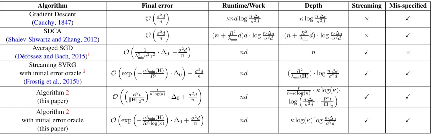
Figure 1: Effect of increased batch sizes on the Algorithm’s generalization error. The variance de-creases monotonically with increasing batch size. The bias indicates that the rate of decay inde-creases till the optimalbthresh. Withb =bthresh, mini-batch SGD obtains the same generalization error as
batchsize1using smaller number of iterations (i.e. smaller depth) compared to larger batch sizes.
Lemma 8 Consider the well-specified case of the streaming LSR problem. With a batch sizeb, step sizeγ =γb,max/2, the limiting centered varianceηvariance∞ has an expected covariance that is upper bounded in a psd sense as:
Eηvariance∞ ⊗ηvariance∞
1
R2+ (b−1)kHk 2
·σ2·I.
Characterizing the behavior of the final iterate is crucial towards obtaining bounds on the behavior of the tail-averaged iterate. In particular, the final iterate having a excess variance riskO(σ2)(as is the case with lemma (8)) appears crucial towards achieving minimax rates of the averaged iterate.
5. Experimental Simulations
We conduct experiments using a synthetic example to illustrate the implications of our theoretical results on mini-batching and tail-averaging. The data is sampled from a50− dimensional Gaus-sian with eigenvalues decaying as{1
k} 50
k=1 (condition numberκ = 50), and the varianceσ2 of the (additive noise) noise is 0.01. In this case, our estimated batch size according to Theorem 1 is
bthresh = 11. Our results are presented by averaging over 100independent runs of the Algorithm, and each run employs200κsamples. All plots are log-log with x-axis being the depth, and y-axis the excess risk. For our plots, we assume that each iteration takes constant time for all batch sizes; this is done to present evidence regarding the tightness of our mini-batching characterization limits that yield linear parallelization speedups over SGD with mini-batch size of1.
We consider the effect of mini-batching (in figure 1) with batch sizes of 1, 3, bthresh = 11,
2·bthresh = 22andd= 50. Averaging begins after observing a fixed number of samples (set as5κ). We see that the rate of bias decay (figure1a) increases until reaching a mini-batch size ofbthresh,
saturating thereafter; this implies we are inefficient in terms of sample size. As expected, the rate of decay of variance (figure1b) is monotonic as a function of mini-batch size. Finally, the overall error (figure1c) shows the tightness of our mini-batching characterization: with a batch size of bthresh,
100 101 102 103
Depth
10-25 10-20 10-15 10-10 10-5
100
(Excess) Bias Risk
start quarterway halfway unaveraged
(a) Bias Risk
100 101 102 103
Depth 10-5
10-4 10-3
10-2
(Excess) Variance Risk
start quarterway halfway unaveraged
(b) Variance Risk
100 101 102 103
Depth 10-5
10-4 10-3 10-2
10-1 100
Total (Excess) Risk
start quarterway halfway unaveraged
(c) Total Risk
Figure 2: [Zoom in to see detail] Effect of tail-averaging with mini-batch size ofbthresh= 11.
In the next experiment, we fix batch size=bthreshand consider the effect of when tail-averaging begins (figure2). We consider averaging iterates from the start (as prescribed byD´efossez and Bach (2015)), after a quarter/half of total number of iterations, and unaveraged SGD as well. We see that the bias (figure2a) exhibits a geometric decay in the unaveraged phase while switching to an slower
O(t12)rate with averaging. The variance (figure2b) tends to increase and stabilize atO( σ2
bthresh)in the
absence of averaging, while switching to aO(N1) decay rate when averaging begins. The overall generalization error (figure2c) shows the superiority of the scheme where averaging after a burn-in period allows the bias to decay towards the noise level at a geometric rate, following which tail-averaging allows us to decay the variance term, providing credence to our theoretical results that tail-averaged SGD allows us to obtain better generalization error as a function of sample size.
6. Concluding Remarks
This paper analyzes several algorithmic primitives often used in practice in conjunction with vanilla SGD for the stochastic approximation problem. In particular, this paper provides a sharp non-asymptotic treatment of (a) mini-batching, (b) tail-averaging, (c) effects of model mismatch, (d) behaviour of the final iterate, (e) highly parallel SGD method based on doubling batch sizes and (f) model-averaging/parameter mixing schemes for the strongly convex streaming LSR problem.
The effect of mini-batching and other algorithmic primitives mentioned above can be stood for a variety of models and/or algorithms. In particular, future directions could include under-standing these issues for stochastic approximation with the Logistic Loss (Bach,2014), streaming PCA (Jain et al.,2016a), and other algorithms such as streaming SVRG (Frostig et al.,2015b).
Acknowledgments
Appendix A. Appendix
We begin with a note on the organization:
• SectionA.1introduces notations necessary for the rest of the appendix.
• SectionA.2derives the mini-batch SGD update and provides the bias-variance decomposition and reasons about its implication in bounding the generalization error.
• SectionA.3provides lemmas that are used to bound the bias error.
• SectionA.4provides lemmas that are used to bound the variance error.
• SectionA.5uses the results of the previous sections to obtain the main results of this paper.
A.1 Notations
We begin by introducing the centered iterateηti.e.:
ηtdef= wt−w∗.
In a manner similar towt, the tail-averaged iteratewt,N is associated with its corresponding
cen-tered estimateη¯t,N def= wt,N−w∗= N1 Pts+=Nt−1(ws−w∗) = N1 Pst+=Nt−1ηs. Next, letΦtdenote the expected covariance of the centered estimateηt, i.e.
Φt def
= E[ηt⊗ηt],
and in a similar way as the final iteratewt, the tail-averaged estimatewt,N is associated with its
expected covariance, i.e.Φ¯t,N def
= Eη¯t,N ⊗η¯t,N
.
A.2 Mini-Batch Tail-Averaged SGD: Bias-Variance Decomposition
In sectionA.2.1, we derive the basic recursion governing the evolution of the iterateswtand the tail-averaged iteratews+1,N. In sectionA.2.2we provide the bias-variance decomposition of the final iterate. In sectionA.2.3, we provide the bias-variance decomposition of the tail-averaged iterate.
A.2.1 THE BASIC RECURSION
At each iterationtof Algorithm1, we are provided withbfresh samples{(xti, yti)}bi=1drawn i.i.d. from the distributionD. We start by recounting the mini-batch gradient descent update rule that allows us to move from iteratewt−1towt:
wt=wt−1−
γ b
b
X
i=1
(hwt−1,xtii −yti)xti,
where, 0 < γ < γb,max is the constant step size that is set to a value less than the maximum
allowed learning rateγb,max. We also recount the definition ofwt,N which is the iterate obtained by averaging forN iterations starting from thetthiteration, i.e.,
wt,N =
1
N
t+N−1 X
s=t
Let us first denote the residual error term by i = yi − hw∗,xii. By the first order optimality conditions ofw∗, we observe thatandxare orthogonal, i.e,E(x,y)∼D[·x] = 0. For any estimate w, the excess risk/generalization error can be written as:
L(w)−L(w∗) = 1
2Tr
H· η⊗η
, withη=w−w∗. (11)
We now write out the main recursion governing the mini-batch SGD updates in terms ofη.:
ηt=
I− γ b
b
X
i=1
xti⊗xti
ηt−1+
γ b
b
X
i=1
tixti
=I− γ
b
b
X
i=1
xti⊗xti
ηt−1+ γ
b
b
X
i=1
ξti
=Ptbηt−1+γζtb, (12)
where, Ptb def
= I− γb Pb
i=1xti ⊗xti
andζtb def= 1bPb
i=1ξti = 1b
Pb
i=1tixti. Equation 12 automatically brings out the “operator” view of analyzing the (expected) covariance of the centered estimateΦt = E[ηt⊗ηt] to provide an estimate of the generalization error. We now note the following about the covariance ofζtb:
E[ζtb⊗ζt0b] =
1
b2 X
i,j
E[ξti⊗ξt0j]
= h1
b2 b
X
i=1
E[ξti⊗ξti]
i
1[t=t0] = 1
bΣ 1[t=t 0
], (13)
where,1[.]is the indicator function, and equals1if the argument inside[.]is true and0otherwise. We note that the expectation of the cross terms in equation13is zero owing to independence of the samples{xti, yti}bi=1as well as between{xti, yti}bi=1, {xt0i, yt0i}b
i=1∀t6=t
0and owing to the first
order optimality conditions. Owing to the invariance ofζtb on the iterationt, context permitting, we sometimes drop the iteration indextfromζtband simply refer to it asζb.
Next we expand out the recurrence (12). Let Qj,t = (Qtk=jPkb)T with the convention that
Qt0,t=I∀t0> t. With this notation we have:
ηt=Ptbηt−1+γζtb
=PtbPt−1,b...P1,bη0+γ
t−1 X
j=0
{Ptb....Pt−j+1,b}ζt−j,b
=Q1,tη0+γ
t−1 X
j=0
Qt−j+1,tζt−j,b
=Q1,tη0+γ
t
X
j=1
Qj+1,tζj,b
where, we note that
ηbiast def= Q1,tη0 (15) relates to understanding the behavior of SGD on the noiseless problem (i.e. ζ·,·= 0a.s.) and aims
to quantify the dependence on the initial conditions. Further,
ηvariancet def= γ
t
X
j=1
Qj+1,tζj,b (16)
relates to the behavior of SGD when begun at the solution (i.e. η0 = 0) and allowing the noiseζ·,·
to drive the process.
Furthermore, considering the tail-averaged iterate obtained by averaging the iterates of the SGD procedure for N iterations starting from a certain number of iterations “s”, i.e., we examine the quantityη¯s+1,N = ws+1,N −w∗, wherews+1,N = N1 Pst=+sN+1wt. We write out the expression forη¯s+1,Nstarting out from equation14:
¯
ηs+1,N = 1
N
s+N
X
t=s+1
ηt
= 1
N
s+N
X
t=s+1
ηbiast +ηvariancet (from equation14)
= ¯ηbiass+1,N+ ¯ηvariances+1,N. (17)
A.2.2 THEFINALITERATE: BIAS-VARIANCEDECOMPOSITION
The behavior of the final iterate is considered to be of great practical interest and we hope to shed light on the behavior of this final iterate and the tradeoffs between the learning rate and batch size. Since the generalization error of any iteratewN obtained by running mini-batch SGD with a batch sizebfor a total ofNiterations can be estimated by trackingE[ηN⊗ηN], where,ηN =wN−w∗, we provide a simple psd upper bound on the outer product of interest, i.e.:
E[ηN⊗ηN] =E
ηbiasN +ηvarianceN ⊗ ηbiasN +ηvarianceN (by substituting equation14)
2·
E ηbiasN ⊗ηbiasN
+E ηvarianceN ⊗ηvarianceN
.
Using this expression, we now write out the expression for the excess risk of the final iterate:
E[L(wN)]−L(w∗) =
1
2hH,E[ηN ⊗ηN]i
≤ 1
2hH,2· E
ηbiasN ⊗ηbiasN
+EηvarianceN ⊗ηvarianceN i
≤2·
1
2hH,E
ηbiasN ⊗ηbiasN
i+1
2hH,E
ηvarianceN ⊗ηvarianceN
i
= 2·
EL(wNbias)
−L(w∗)+ EL(wvarianceN )
−L(w∗)
A.2.3 THETAIL-AVERAGEDITERATE: BIAS-VARIANCEDECOMPOSITION
Now, considering the fact that the excess risk/generalization error (equation 11) involves track-ingEη¯s+1,N⊗η¯s+1,N
, we see that the quantity of interest can be bounded by considering the behavior of SGD on bias and variance sub-problem. In particular, writing out the outerproduct of equation17, we see the following inequality holds through a straightforward application of Cauchy-Shwartz inequality:
Eη¯s+1,N ⊗η¯s+1,N
2· Eη¯biass+1,N⊗η¯biass+1,N
+Eη¯variances+1,N ⊗η¯variances+1,N
). (19)
The above equation is referred to as the bias-variance decomposition and is well known from previ-ous work on Stochastic Approximation (Bach and Moulines,2013;Frostig et al.,2015b;D´efossez and Bach,2015). This implies that an upper bound on the generalization error (equation11) is:
L(ws+1,N)−L(w∗) =
1
2hH,E
¯
ηs+1,N⊗η¯s+1,N
i
≤ hH,Eη¯biass+1,N⊗η¯biass+1,N
i+hH,Eη¯svariance+1,N ⊗η¯variances+1,N
i. (20)
Here, we adopt the proof approach ofJain et al.(2017a). In particular,Jain et al.(2017a) provide a clean way to simplify the expression corresponding to the tail-averaged iterate. Let us consider
Eη¯s+1,N⊗η¯s+1,N
and simplify the resulting expression: in particular,
E
h ¯
ηs+1,Nη¯>s+1,Ni= 1
N2 s+N
X
l=s+1 s+N
X
k=s+1
E[ηl⊗ηk]
= 1
N2 ·
X
l≥k
E[ηl⊗ηk] +
X
l<k
E[ηl⊗ηk]
1
N2 ·
X
l≥k
E[ηl⊗ηk] +
X
l≤k
E[ηl⊗ηk]
(∗)
= 1
N2 ·
X
l≥k
(I−γH)l−kE[ηk⊗ηk] +
X
l≤k
E[ηl⊗ηl] (I−γH)k−l
(∗∗)
= 1
N2 · X
l≤k
E[ηl⊗ηl] (I−γH)k−l+ (I−γH)k−lE[ηl⊗ηl]
= 1
N2 · s+N
X
l=s+1 s+N
X
k=l
E[ηl⊗ηl] (I−γH)k
−l+ (I−γH)k−l
E[ηl⊗ηl]
= 1
N2 · s+N
X
l=s+1
∞
X
k=l
E[ηl⊗ηl] (I−γH)k−l+ (I−γH)k−lE[ηl⊗ηl]
− 1 N2 ·
s+N
X
l=s+1
∞
X
k=s+N+1
E[ηl⊗ηl] (I−γH)k−l+ (I−γH)k−lE[ηl⊗ηl]
= 1
N2 · s+N
X
l=s+1
E[ηl⊗ηl] (γH)−1+ (γH)−1E[ηl⊗ηl]
− 1 N2
s+N
X
l=s+1
∞
X
k=s+N+1
E[ηl⊗ηl] (I−γH)k−l+ (I−γH)k−lE[ηl⊗ηl]
(∗ ∗ ∗), (21)
where,(∗)is a valid PSD upper bound as we add and subtract the diagonal terms{E
ηkη>k
}sk+=Ns+1.
(∗∗)follows because of the following (assumel > k; the other case follows similarly):
E[ηl⊗ηk] =E
Plbηl−1+γζlb
⊗ηk
=EE Plbηl−1+γζlb
⊗ηk|Fl−1
=EE Plbηl−1+γζlb
|Fl−1
⊗ηk
= (I−γH)Eηl−1⊗ηk
,
where, the final equation follows sinceE[Plb|Fl−1] =E
h
I−γb Pb
i=1xli⊗xli|Fl−1 i
=I−γH
and E[ζlb|Fl−1] = 0 from first order optimality conditions. Recursing over l yields the result.
(∗ ∗ ∗)follows from summing a (convergent) geometric series.
This implies that the excess risk corresponding to the bias/variance term can be obtained from equation21by taking an inner product withH, i.e.:
hH,Eη¯s+1,N⊗η¯s+1,N
i ≤ 1 N2 ·
s+N
X
l=s+1
hH,E[ηl⊗ηl] (γH)
−1+ (γH)−1
E[ηl⊗ηl]i
− 1 N2 ·
s+N
X
l=s+1
∞
X
k=s+N+1
hH,E[ηl⊗ηl] (I−γH)k−l
+ (I−γH)k−lE[ηl⊗ηl]i
≤ 1 N2 ·
s+N
X
l=s+1
hH,E[ηl⊗ηl] (γH)−1+ (γH)−1E[ηl⊗ηl]i
= 2
γN2 · s+N
X
l=s+1 Tr
E[ηl⊗ηl]
. (22)
The upper bound on the final line follows because each term within the summation in the second line is negative owing to the following argument. Consider say,
hH,E[ηl⊗ηl] (I−γH)k−l+ (I−γH)k−lE[ηl⊗ηl]i
= 2 Tr
H(I−γH)k−lE[ηl⊗ηl]
≥0.
Note thatHand(I−γH)commute and both are psd, implying thatH(I−γH)k−lis PSD. Finally, the trace of the product of two PSD matrices is positive withH(I−γH)k−lbeing one of these PSD matrices andE[ηl⊗ηl]being the other, thus yielding the claimed bound in equation22.
This implies that the overall error (through equation11) can be upperbounded as:
E[L(ws+1,N)]−L(w∗) =
1
2· hH,E
¯
≤ 1 γN2
s+N
X
l=s+1
Tr E[ηl⊗ηl]
≤ 2 γN2 ·
s+N
X
l=s+1
Tr Eηbiasl ⊗ηbiasl + Tr E
ηvariancel ⊗ηvariancel
,
(23)
where the final line follows from equation19. We will now bound each of these terms to precisely characterize the excess risk of mini-batch averaged SGD. We refer to the bias error of the tail-averaged iterate as the following:
EL(wbiass+1,N)
−L(w∗)def= 2
γN2 s+N
X
l=s+1 Tr
Eηbiasl ⊗ηbiasl
. (24)
Similarly, we refer to the variance error of the tail-averaged iterate as the following:
EL(wvariances+1,N)
−L(w∗)def= 2
γN2 s+N
X
l=s+1 Tr
Eηvariancel ⊗ηvariancel
. (25)
A.3 Lemmas For Bounding The Bias Error Lemma 9 Withγ ≤ γb,max
2 =
b R2·ρ
m+(b−1)kHk2, the following bound holds:
E
(I− γ b
b
X
j=1
xli⊗xli)(I−
γ b
b
X
j=1
xli⊗xli)
2
≤1−γµ.
Proof This lemma generalizes one appearing inJain et al. (2017a) to the mini-batch size bcase. Denote byUthe matrix of interest and consider the following:
U=E
(I−γ b
b
X
j=1
xli⊗xli)(I−
γ b
b
X
j=1
xli⊗xli)
=I−γH−γH+
γ b 2 · bE h
kxk2xx>
i
+b(b−1)H2
I−2γH+γ 2
b · R
2H+ (b−1)kHk 2
H
=I−γH,
from which a spectral norm bound implied by the lemma naturally follows.
Lemma 10 For any learning rateγ ≤γb,max/2, the bias error of the tail-averaged iteratewbiass+1,N is upper bounded as:
EL(wbiass+1,N)
−L(w∗)≤ 2
γ2N2µ2(1−γµ)
s+1· L(w
0)−L(w∗)
![Figure 2: [Zoom in to see detail] Effect of tail-averaging with mini-batch size of bthresh = 11.](https://thumb-us.123doks.com/thumbv2/123dok_us/9791428.1964863/18.612.91.521.92.222/figure-zoom-effect-tail-averaging-mini-batch-bthresh.webp)
