R E S E A R C H
Open Access
A Bayesian network approach to the database
search problem in criminal proceedings
Alex Biedermann
1*, Jo¨elle Vuille
2and Franco Taroni
1Abstract
Background: The ‘database search problem’, that is, the strengthening of a case in terms of probative value -against an individual who is found as a result of a database search, has been approached during the last two decades with substantial mathematical analyses, accompanied by lively debate and centrally opposing conclusions. This represents a challenging obstacle in teaching but also hinders a balanced and coherent discussion of the topic within the wider scientific and legal community. This paper revisits and tracks the associated mathematical analyses in terms of Bayesian networks. Their derivation and discussion for capturing probabilistic arguments that explain the database search problem are outlined in detail. The resulting Bayesian networks offer a distinct view on the main debated issues, along with further clarity.
Methods: As a general framework for representing and analyzing formal arguments in probabilistic reasoning about uncertain target propositions (that is, whether or not a given individual is the source of a crime stain), this paper relies on graphical probability models, in particular, Bayesian networks. This graphical probability modeling approach is used to capture, within a single model, a series of key variables, such as the number of individuals in a database, the size of the population of potential crime stain sources, and the rarity of the corresponding analytical characteristics in a relevant population.
Results: This paper demonstrates the feasibility of deriving Bayesian network structures for analyzing, representing, and tracking the database search problem. The output of the proposed models can be shown to agree with existing but exclusively formulaic approaches.
Conclusions: The proposed Bayesian networks allow one to capture and analyze the currently most well-supported but reputedly counter-intuitive and difficult solution to the database search problem in a way that goes beyond the traditional, purely formulaic expressions. The method’s graphical environment, along with its computational and probabilistic architectures, represents a rich package that offers analysts and discussants with additional modes of interaction, concise representation, and coherent communication.
Keywords: Database search, Evidential value, Bayesian approach, Bayesian networks
Background
The emergence of DNA databases from a legal point of view DNA is widely held as a category of forensic trace mate-rial that outperforms other forensically relevant matemate-rial on parameters such as reliability. This is reflected by opin-ions maintained by both members of the general public and professional and academic areas, and exemplified by
*Correspondence: [email protected]
1School of Criminal Justice, Institute of Forensic Science, University of Lausanne, Lausanne, 1015, Switzerland
Full list of author information is available at the end of the article
expressions such as ‘silver bullet’ [1], the ‘most powerful innovation in forensics since fingerprinting’ [2], or a ‘per-fect piece of evidence’ [3]. Databases represent a transient topic in that respect. Historically, modern DNA analy-ses were first used as an investigative tool in an English criminal case in 1986, when Colin Pitchfork was pros-ecuted and convicted for the rape and murder of two teenage girls. In the absence of a suspect, the police tested more than 4,000 males from the region of interest (a procedure known today as mass screening). The investi-gation finally came upon Pitchfork - who refused to give blood for analysis arguing that he was afraid of needles
- only after that considerable resources and time had been spent. At the time, DNA clearly lacked the element that gives it the formidable investigative capacities it has today: databases.
The first DNA profile databases were established during the 1990sa. Since then, all major Western countries have enacted laws allowing the establishment of DNA profile databases, but the exact conditions under which they function vary from one jurisdiction to another. Besides, they are still accompanied by or cause democratic debate as to whose DNA profile should be taken and kept regis-tered. While databases may be seen as a natural byproduct of DNA typing, they now are used daily without many lawyers or even scientists devoting in-depth thought to the way a search through a database could influence the value of the DNA evidence itself. Forensic academics though have been struggling for at least a decadebover the
meaning of a match found through ‘trawling a database’ versus situations where suspects were found through other investigative means (that is, without the use of database).
The outcomes of this debate, at times led rather con-troversially, are approached in this article from a distinct perspective of a graphical approach. As a principal aim, the discussion will focus on explaining how the use of a database impacts the value assigned to a ‘match’ between the profile of a trace found on the scene of a crime and the profile of a suspect. This question appears to have no intuitively obvious answer, and it may seem overly tech-nical to lawyers and other legal academics, but, as further emphasized in due course, it is in their interest to under-stand the challenges raised by DNA databases in terms of formal and argumentative interpretation procedures and the impact that this may have on their area of activity.
This pairs with the more general tendency that the use of databases has fundamentally changed the way forensic evidence is currently processed, to the extent that, con-trary to more traditional modes of proof, the judiciary tends to lose control over a whole part of the administra-tion of the evidence [4]. So to speak, and as a matter of fact, a database can be viewed as a ‘closed box’ because its actual inner workings remain unknown not only to most defense lawyers, but also to many representatives of the judiciary, namely prosecutors, judges, and juries. Besides the challenge of interpreting the probative value of the so-called ‘database hits’, the way in which a database is man-aged, the way that the correctness of typing results and registrations are controlled, or the way databases are used for calculating so-called ‘rarity statistics’ are all topics that remain largely outside the control of judicial actors. This is problematic because it may lead to unawareness that such questions could be debated and that the probative value of matches reported to legal actors are intrinsically linked to such issues.
From a more general point of view, questioning the inferential assessment of database search results is a sub-ject all the more relevant because databases are growing continuously larger. With more people being registered every year, database searching of DNA profiles from traces of unknown origin involves comparisons with increas-ingly larger stocks of data. This motivates investigation of the knowledge, perception, and understanding of this situation, along with its practical implications in judicial proceedings. In the UK, for example, about 5% of the populationchave had their profile taken and entered into the national DNA database, which not only comprises profiles from convicted and serious offenders, but also from people implicated in minor cases. Yet, the probabil-ity of finding a correspondence with an individual that is not the true source is not equal to zero. With a potential of adventitious matches, each database member thus runs a real risk to face a charge based on a ‘database hit’. For these reasons, questions that emanate from the use made of matches derived from database searches, as well as the assessment of their evidential value, are crucial and a topic that represents ongoing interest to the legal community.
and can decide according to their temporary states of mind, that is, their mere mood. In fact, the law requires decision makers to proceed in a rational way, so as to avoid unfair or arbitrary decisions.
This raises the question of what is meant by the notion of rationality in the context of the interpretation of foren-sic evidence. There is widespread agreement, supported by substantive argument, on the view that judges or juries should follow the rules of logic and of common scien-tific knowledge and that Bayesian reasoning provides a coherent framework to conform with this requirement [6-8]. This approach - of which Bayesian networkseare a schematic illustration and retained as such in this paper - assists decision makers in their assessment of situations in the light of new pieces of evidence, but it does not, in itself, instruct its user about the actual probative value that ought to be given to, for instance, a DNA match. Once a match has been reported, it rather defines the general rules according to which one’s beliefs should evolve in view of the uncertain target propositions, such as that according to which a given suspect is or is not the source of a stain found on the crime scene. Applying Bayes’ inference in a particular situation requires one to specify a model. This will be the main topic of discussion pursued in the section “The ‘island’ problem” and in later parts of this paper.
Evidential value of ‘database hits’: two decades of debate ‘What is the strength of the evidence against a suspect who is found as a result of the search in a database?’ This practical question, also sometimes referred to as ‘the database search problem’, has led to considerable dis-cussion within the scientific community, including both forensic scientists and legal practitioners. Its implica-tions in the practice of criminal proceedings span a wide range. The debate was led essentially in the context of DNA evidence, but the underlying principle of searching databases containing analytical characteristics that serve as a basis for comparative forensic examinations applies also to other kinds or categories of scientific evidence [9]. Although this problem is strongly rooted in prac-tical applications, deciding on an appropriate approach to deal with this inference problem requires coherent methodological developments.
Different answers, pointing in quite contrary directions, have been offered so far but are accompanied with sub-stantial mathematics. It is not the paper’s intention to retrace this debate in all its respects nor to oppose com-peting approaches. As a starting point, it suffices to note that the prevalent and most well-supported viewpoint is that a database search tends to strengthen a case against a ‘matching’ suspect [10-18]. This paper seeks to analyze and discuss the probabilistic tenets on which this stand-point is founded by invoking a methodology based on
graphical probability models (that is, Bayesian networks). Some work in this direction has already been presented in [19,20]. A more recent paper also relied on Bayesian networks [21], but its main focus was on a slightly dif-ferent aspect, that is, the probability of false convictions. This paper will concentrate on the more restricted topic of how to infer the source of a crime stain. As will be seen, a graphical approach using Bayesian networks allows to demonstrate a logic that is in line with existing literature on this topic.
Structure of the paper
This paper is organized as follows. The ‘Methods’ section starts by providing general information about Bayesian networks and explains the rationale behind their use as a methodology in the study reported here. As an introduc-tory example and an initial finding, “The ‘island’ problem” section presents a Bayesian network approach for the well-known ‘island problem’. This is a generic setting in which no database is involved [22]. The discussion thus seeks to introduce the graphical structure of probabilistic reasoning about the source of a crime stain in a situation where the use of a database is not an issue. This start-ing point is chosen in order to illustrate the logic of the extended argument that is - in later parts of the paper - developed for situations in which the profiles of some of the islanders are placed in a searchable database. This allows to point out the logical connection between these two evaluative scenarios. As will be seen, there are struc-tural analogies between the two analyses, and this gives further credit to the proposed solution for the database setting. In particular, it will be possible to show that the approach to the database search problem is merely a log-ical extension of the undisputed probabilistic solution to the island problem. In addition, the graphical interface of Bayesian networks will be shown to provide a clear, yet intuitively convincing explanation for an increase of the probability of the proposition according to which a match-ing suspect is the source of the crime stain, once other members of the same database are excluded (because they are found to present non-matching profiles).
can also serve the purpose of illustrating the derivation of a likelihood ratio. This aspect is introduced because the previous sections mainly focused on the calculation of posterior probabilities for main propositions (for exam-ple, ‘the suspect is the source of the crime stain’). The merit of a Bayesian network-guided analysis for both pos-terior probabilities and likelihood ratios is discussed in the ‘Discussion and conclusions’ section, along with general conclusions. Throughout the paper, the level of techni-cality for notation and calculation does not exceed that which is generally employed in existing legal literature on the topic, for example [18], but readers who wish to avoid the derivation of the mathematical background in order to concentrate on the proposed Bayesian networks may focus directly on the following sections: ‘Bayesian network for the island problem,’ ‘Bayesian network for a database search setting: suspect and one other individual in the database,’ ‘Bayesian network for a search of a database of sizen>2,’ and ‘Discussion and conclusions’.
Methods Preliminaries
In the early 1980s, Bayesian networks have been devel-oped in the field of artificial intelligence as an approach that helps to apply the theory of probability to inference problems of more substantive size and, thus, to more real-istic and practical problems [23]. Since then, Bayesian networks have also attracted researchers in legal sciences, and this tendency has considerably intensified through-out the last decade [24]. Aitken and coauthors [25,26], for example, investigated the potential of Bayesian networks for specific case analysis, also known as ‘offender profiling’. Based on a dataset covering the details of several hundred cases of sexually motivated child murders and abduc-tions (that is, incidents reported in Great Britain since 1960), the authors propose different graphical models to relate the key parameters of a case. These models may be used to revise the probability of offender characteris-tics, given the information about the victim and the crime. More recently, the use of Bayesian networks has also been reported for crime risk factor analysis [27] as well as for terrorism risk management [28]. Within forensic science, they now constitute a major direction of research [20]. Beyond legal applications, such as the modeling of his-torically causes c´el`ebres [29-32], Bayesian networks are used in virtually any field that needs to deal with inference under circumstances of uncertainty (for example, medical diagnosis, engineering).
Methodology
In this paper, a Bayesian network approach is proposed because it allows one to point out the logic underlying current probabilistic analyses of the database search prob-lem in various ways. Making these arguments plain is
relevant not only for teaching, but also for supporting dis-cussion within the scientific community. There is a need for this essentially because the developments based on formulae alone may not be found easy to apprehend by all participants within a discussion. Yet, agreement on such evaluative matters is essential in order to assure that the forensic community can take a credible stance with respect to recipients of expert information, in particu-lar, legal decision makers (such as magistrates or courts of law). Moreover, there are also recent recommenda-tions from professional bodies, for example [33], that diverge from the prevalent viewpoint stated above. This is a cause of concern and illustrates the continuing need for formalisms that provide support in analyzing and communicating probabilistic approaches [21].
Results and discussion The ‘island’ problem
General description and notation
Consider a biological stain found on a crime scene. It has been typed and found to have the genetic profile Gc. It
is assumed here that the method applied for determining the genetic profile of a biological sample works perfectly accurate. The ‘island’ on which the crime was committed has a population of sizeN. Initially, there is no informa-tion that directs suspicion to any of theNislanders. Thus, all of them are equally believed to be the source of the crime stain. Since the stain is found to be of typeGc, so
must be the person from which the stain comes. A suspect comes to police attention and his blood is analyzed. He is found to have the genetic profileGs. It corresponds to that
observed for the crime stain:Gc=Gs. On the basis of this
information, the question of interest is as follows: ‘How convinced should one be that the suspect is the source of the crime stain?’
In order to approach this question, information about the occurrence of the corresponding genetic profile is needed. Let us suppose that, on the basis of a survey of a comparable population on another island, the target profile can be taken to occur in about 1% of the popu-lation and that this rate, written asγ for short, can also be retained for the population of the island on which the crime stain of interest was found. It is also supposed here that knowledge of the suspect’s genotype, Gs, does
not affect one’s probability that another islander has that profile.
The formal analysis of this inference problem requires some further notation. Within the population ofN indi-viduals, let us index the suspect as person 1 and the remaining individuals as 2...N. Next, let the proposition that a given personiis the source of the crime stain be denoted as Hi. The term H1 thus stands for the
the remainingN−1 people is the source of the crime stain are denoted asH2, ...,HN. Throughout this paper,
propo-sitions will be abbreviated with capital letters, whereas probability assignments will be written shorthand by Greek symbols.
The initial probability that a given individual is the source of the crime stain will be written asPr(Hi) = πi.
Since it is considered, as a starting point, that each of theN persons could be the source with equal probability, one hasπi = 1/NandNi=1πi = 1. In later sections, further notation is introduced in order to allow for the possibility that some of theNindividuals are part of a database.
Probability that the suspect is the source of the crime stain In the setting considered at this point, the suspect is the only typed individual among the N persons. Let us write M1 for the finding that his genotype, Gs,
corre-sponds to that of the crime stain,Gc. The probability that
the suspect is the source of the crime stain is then given by Bayes’ theorem for discrete evidence and multiple discrete propositions:
Pr(H1|M1)=
Pr(M1|H1)Pr(H1)
Pr(M1|H1)Pr(H1)+Ni=2Pr(M1|Hi)Pr(Hi)
.
(1)
Here, the conditional probability of the evidence M1
given H1 is also called the likelihood of the
propo-sition given the evidence, sometimes written as L1.
Equation 1 can thus be given in a more compact form:
Pr(H1|M1)=
L1π1
L1π1+Ni=2Liπi
. (2)
The likelihood for any personiother than the suspect, that is, the conditional probability of the observed corre-spondence given that some person other than the suspect is the source of the crime stain, depends on the occurrence of the corresponding features in the population:Pr(M1 |
Hi) = Li = γ, fori = 1. Moreover, the probability that
some person other than the suspect is the source of the crime stain is the complement of the probability that the suspect is the source. Therefore,Ni=2πi = 1−π1. The
termNi=2Liπican thus be rewritten as follows:
N
i=2
Liπi= N
i=2
γ πi=γ N
i=2
πi=γ (1−π1).
Assuming that the suspect will certainly match if he is in fact the source of the crime stain,Pr(M1|H1)=L1=1,
the posterior probabilityπ1that the suspect is the source of the crime stain, after considering the evidenceM1, thus
is as follows:
π1 =Pr(H1|M1)=
π1
π1+γ (1−π1) . (3)
Bayesian network for the island problem
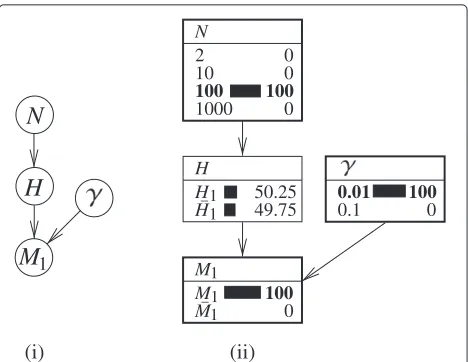
The result from the previous section can be tracked in a Bayesian network as shown in Figure 1i.
This model contains the following elements:
1. NodeN. This is a numeric node with
states2, 10, 100, and 1,000 (other numbers may obviously be chosen) and represents the size of the suspect population, that is, the individuals which could have left the crime stain.
2. NodeH. This node has two states. The stateH1 represents the proposition ‘The suspect is the source of the crime stain’. The stateH¯1represents the composite proposition ‘one of the otherN−1 individuals is the source of the crime stain’. It is an aggregation of all propositionsHi(fori=2, ...,N). The probability table of nodeHcontains
probabilityπ1=1/Nfor the stateH1
and(N−1)/N(which is equivalent to (1−π1)) for the stateH¯1(see Table 1).
3. Nodeγ. This node contains numeric states that represent the rate at which the corresponding genetic feature appears in the population. For the purpose of illustration, the values0.01and0.1are chosen. Notice that this node is not strictly
1
H
1
M
N
2 10
100
1000
N
H H
M M
0.1
0.01
0 0 0
0
0
1 1
1
1 100
100
M
100
49.75 50.25
H_
_
(i) (ii)
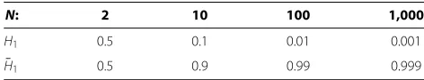
Table 1 Probability table for nodeH
N: 2 10 100 1,000
H1 0.5 0.1 0.01 0.001
¯
H1 0.5 0.9 0.99 0.999
Conditional probabilities assigned to the statesH1andH¯1of the nodeH.
necessary. It would also be possible to specifyγ directly in the probability table of the nodeM1. A representation ofγ in terms of a distinct node is retained here for the reason of providing a detailed decomposition of the problem at hand.
4. NodeM1. This node has two statesM1(‘The suspect’s profile corresponds to that of the crime stain’) andM¯1(‘The suspect’s profile does not correspond to that of the crime stain’). If the suspect is in fact the source of the crime stain (that is, propositionH1holds), then the correspondence,M1, is assumed to occur with certainty (irrespective of the rarity of the corresponding characteristic, expressed byγ). Otherwise (that is,H¯1being true), the correspondence occurs as a function of the rateγ with which the corresponding feature appears in the population. The probability table of the nodeM1 thus completes as shown in Table 2.
An important aspect of the current development is that the scientific evidence is confined solely to the fact that the suspect’s profile is found to correspond with the profile of the crime stain. Nothing is said about how mem-bers of the remaining N−1 individuals compare to the crime stain.
For the purpose of illustration, let us assume that the size of the suspect population is N = 100, and the rate γ at which the corresponding genetic characteris-tic occurs in the population is 0.01. Further, according to Equation 3 and assuming a prior probability of 1/Nfor each of theN individuals, the probability that the stain comes from the suspect is 0.01/(0.01+0.01×(1−0.01))=
0.5025. This result can also be found via the proposed Bayesian network. A visual illustration of this is given in Figure 1ii. The instantiated nodes (that is, nodes set to the state ‘known’) are shown in bold. The target probability, Pr(H1|M1), is displayed in the nodeH.
Table 2 Probability table for nodeM
H: H1 H¯1
γ: 0.01 0.1 0.01 0.1
M1 1 1 0.01 0.1
¯
M1 0 0 0.99 0.9
Conditional probabilities assigned to the statesM1andM¯1of the nodeM.
When some islanders are in a database Formal analysis
The island problem as described in the previous section is now slightly modified. It will still be assumed that the variable N represents the size of the total population. However, the analysis will suppose that the DNA profiles of the first 1, ...,nindividuals (where index 1 is that of the suspect) are in a database. The individuals(n+1), ...,Nare outside the database. Also part of the assumptions in this scenario is that the profile of the crime stain is compared to all nindividuals. This search of the database reveals that only the profile of the suspect corresponds to the pro-file of the crime stain. This correspondence is denoted, as before, by M1. Besides, the database search has also
revealed that the 2, ...,nindividuals on the database other than the suspect do not match. The fact that a profile of an individual i (for i = 2, ...,n) does not correspond to the crime stain is denoted here byXi. We can thus write
X2&X3&...&Xn for the information that all entries of the
database other than that of the suspect do not correspond. The latter two items of evidence need to be jointly eval-uated, so let us write, following [18], the totality of the evidence asEn=M1&X2&X3&...&Xn.
Considering that there are nof theN individuals in a database leads to a minor refinement in the way in which the source level propositions Hi (for i = 2, ...,N) are
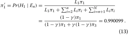
formulated. In fact, they can now be framed as ‘the indi-vidual iin the database is the source of the crime stain’. A more conceptual underpinning of the latter proposi-tions is that they refer to individuals who had their DNA profile compared to that of the crime stain. This is a difference with respect to the individuals (n + 1), ...,N whose profiles were not compared. On the whole, one can thus think of the population of size N as a splitting into nindividuals as database members andN −nthat are not. This splitting becomes apparent when rewriting the posterior probability defined earlier in Equation 1. Writing this probability for the evidence En gives
the following:
Pr(H1|En)=
Pr(En|H1)Pr(H1)
Pr(En|H1)Pr(H1)+ni=2Pr(En|Hi)Pr(Hi) +N
i=n+1Pr(En|Hi)Pr(Hi)
.
(4)
Alternatively, invoking the abbreviated notation, this formula takes the following form:
π1 =Pr(H1|En)=
L1π1
L1π1+ni=2Liπi+Ni=n+1Liπi
.
Since it is still assumed here that the initial probabili-tiesPr(Hi) are given by 1/N, it becomes relevant to draw
attention to the likelihoodsPr(En | Hi)because they will
determine whether or not the posterior probability ofH1
givenEn(Equation 4) is different from the posterior
prob-ability ofH1knowing only the match of the suspect,M1
(Equation 1), and nothing about the matching status of all the individuals other than the suspect.
Consider the following:
1. Pr(En|H1). This term represents the probability that the suspect’s profile corresponds to that of the crime stain and that none of the othern−1members on the database correspond, given that the suspect is the source of the crime stain. The suspect is assumed to match certainly, if he is in fact the source, whereas each of then−1individuals may correspond with probabilityγ. The probability that none of the latter individuals corresponds thus is(1−γ )n−1. We can thus writePr(En|H1)=1×(1−γ )n−1, or
L1=(1−γ )n−1for short.
2. Pr(En|Hi), fori=2, ...,n. This term represents the likelihood for the othern−1individuals in the database. Clearly, given the stated assumptions about the reliability of the typing DNA technique, one would expect to have a match among then−1 individuals on the database if the true source is among them. Therefore, the probability of observingEn, that is, a match with the suspect but with none of the othern−1database members, is zero:Li=0fori=2, ...,n.
3. Pr(En|Hi), fori=n+1, ...,N. This term represents the likelihood for each individual outside the
database. If one of thei=n+1, ...,Nindividuals is the source of the crime stain, then the suspect may match with probabilityγ, and all members on the database other than the suspect will ‘not’ match with probability(1−γ )n−1. Therefore, the likelihood thatLifor each individuali=n+1, ...,N isγ (1−γ )n−1.
Equation 5 thus changes to become the following:
π1 =Pr(H1|En)= L1
π1
L1π1+ n
i=2 Liπi
0
+N i=n+1Liπi
= (1−γ )n−1π1
(1−γ )n−1π
1+Ni=n+1γ (1−γ )n−1πi
.
(6)
In the denominator, the constantγ (1−γ )n−1can be taken out of the sum. In addition,(1−γ )n−1cancels in
both the numerator and the denominator. This leaves one with the following:
π1 =Pr(H1|En)=
π1
π1+γNi=n+1πi
. (7)
The logic of this result is that the second term in the denominator,γNi=n+1πi, is smaller thanγ (1−π1)
in Equation 3. This latter expression involves a sum of prior probabilities over the entire population (with no one except the suspect being in the database) minus the suspect. The former, in Equation 7, involves only a sum over those members of the population which are not in the database. Stated otherwise, the prior probabilities for the individuals in the database which are found to have profiles different from that of the crime stain can-cel because of the multiplication with the zero likelihoodf. Because of a smaller denominator, the posterior probabil-ityπ1 in Equation 7 turns out to be greater than that in Equation 3. The selection of a suspect in a database along with an exclusion of other database members by DNA evi-dence thus reunites more evievi-dence against the matching suspect.
Bayesian network for a database search setting: suspect and one other individual in the database
The Bayesian network earlier described in Figure 1 can serve as a starting point for extending analyses to sit-uations involving the search of a database. In order to point this out in a stepwise procedure, let us start with a situation in which there are only two individuals in the database (n = 2), the suspect and one other person. The following modifications are introduced in the graphical model (see also Figure 2):
1. NodeH. A distinct propositionH2is introduced. It refers to the proposition according to which the individual 2 - the second individual on the database besides the suspect - is the source of the crime stain. As before (section ‘Bayesian network for the island problem’), the propositionH1states that the suspect (that is, the individual indexed as 1) is the source of the crime stain. The previous propositionH¯1, accounting for all individuals in the population of sizeNexcept the suspect, is modified toH3N. This latter proposition specifies that the true source is among theN−nindividuals outside the database (as noted above,n is set to 2 for the time being). The probability table of the nodeHcompletes as follows (n=2):
Pr(H1|N)=Pr(H2|N)=1/N,
2
N
X
M
H
1
Figure 2Bayesian network for assessing a single database ‘hit’.
Structure of a Bayesian network for evaluating a correspondence (M1) between the profile of a crime stain and that of a sample from a suspect when the suspect is on a database along withn−1 other individuals whose DNA profiles do not correspond. The size of the population of potential offenders isN. Among theNindividuals,n (withn<N) are on a database. The nodeHhas three states: ‘the suspect is the source of the crime stain’ (H1), ‘the second individual in the database is the source of the crime stain’ (H2), and ‘the source of the crime stain is among theN−n(here,n=2) individuals outside the database’ (H3N). The corresponding genetic feature occurs in the population with rateγ. The nodeX2is binary and represents the proposition according to which the profile of individual 2 (in the database) does not correspond to the crime stain.
It is still assumed that, initially, each member of the population of sizeNhas the same probability of being the source of the crime stain.
2. NodeX2. This is a newly introduced binary node with statesX2, defined as ‘the profile of individual 2 in the database does not correspond to the crime stain profile’, andX¯2, defined as ‘the profile of individual 2 corresponds to that of the crime stain’. For situations in which individual 2 is not the source of the crime stain, the probability that it will nevertheless be found to correspond depends on the rarity of the characteristic. Therefore, nodeX2 depends on the nodeγ. The probability table for the nodeX2completes as shown in
Table 3.
3. NodeM1. The definition of this node is the same as that given earlier in the section ‘Bayesian network for the island problem’. However, an extension of the probability table is necessary because of the modified states of the nodeH. This is shown in
Table 4.
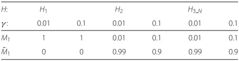
In order to investigate the properties of the proposed Bayesian network, consider again a setting in which the population of potential sources is of sizeN=100, and the
Table 3 Probability table for nodeX2
H: H1 H2 H3N
γ: 0.01 0.1 0.01 0.1 0.01 0.1
X2 0.99 0.9 0 0 0.99 0.9
¯
X2 0.01 0.1 1 1 0.01 0.1
Conditional probabilities assigned to the statesX2andX¯2of the nodeX2.
rarity of the crime stain genotype isγ = 0.01. Introduc-ing the evidenceM1, that is, a correspondence between
the DNA profile of the suspect and that of the crime stain changes the prior probability of Pr(H1) = 1/N = 0.01
into a posterior probability ofPr(H1|M1)=0.5025. This
is a result found earlier in the ‘Bayesian network for the island problem’ section. As shown in Figure 3i, the calcu-lations in the Bayesian network constructed in this section lead to the same finding.
At this point, nothing has been communicated yet to the Bayesian network about whether or not the second individual on the database, besides the suspect, has a cor-responding profile. Notwithstanding, something can be said about the probability that the second individual in the database would match. As shown in Figure 3i, the probability that individual 2 would not match (that is, state X2 being true), given knowledge of M1, is 0.985.
The logic of this result can be derived from the Bayesian network. In fact, that probability is the sum of the prod-ucts of the conditional probabilities of X2 given each
state of the node Hand the actual probabilities of these latter states:
Pr(X2|M1)=Pr(X2|H1)Pr(H1|M1)
+Pr(X2|H2)Pr(H2|M1)
+Pr(X2|H3N)Pr(H3N |M1)
(8)
Given that individual 2 is taken to match with certainty if that individual is in fact the source of the crime stain, one hasPr(X2 | H2) = 0. Consequently, the term in the
center of Equation 8 cancels. Under the remaining propo-sitions, individual 2 matches with probability (1 − γ ). Using shorthand notation for the posterior probabilities
Table 4 Modified probability table for nodeM1
H: H1 H2 H3N
γ: 0.01 0.1 0.01 0.1 0.01 0.1
M1 1 1 0.01 0.1 0.01 0.1
¯
M1 0 0 0.99 0.9 0.99 0.9
1
0
100
X X X
1.50 98.50
2 2
2 1
0
100
0 _
2 10
100
1000
N
0 0 0
100
M _
2
(i)
0.1
0.01
M M1
1 100
M
1
0
_ _
2
X X X2
2 1
0.1
0.01
H
49.49
H
H 50.51
3_N
H
0
(ii)
0
100
2
H
49.25 00.50
H
H 50.25
3_N
H
2 10
100
1000
N
0 0 0
100
M M11
100
Figure 3Expanded representations of a Bayesian network for assessing a single database ‘hit’.Bayesian network (with nodes shown in expanded form) for evaluating a correspondence between the profile of a suspect and that of a crime stain, as defined in Figure 2. Fixed node states are shown in bold. The network(i)shows an evaluation of the information that the suspect’s profile is found to correspond (M1=true) when N=100 andγ=0.01. The posterior probability that the suspect is the source of the crime stain is shown by the stateH1in the nodeH. The network(ii)shows a situation in which the additional information about the second (non-matching) individual on the database is known. Probabilities are shown in percentages.
ofH defined earlier in the text, Equation 8 becomes the following:
Pr(X2|M1) = (1−γ )π1+(1−γ )π3N
= (1−γ )(π1+π3N)
= 0.99×(0.5025+0.4925)=0.9850 .(9)
As a next step in analyzing the proposed Bayesian net-work, one can consider the incorporation of knowledge about individual 2. For the purpose of the current discus-sion, assume that this person is found not to correspond. This amounts to consideringX2 to be true. Introducing
this information into the Bayesian network leads to the result shown in Figure 3ii. As may be seen, the probabil-ity that the suspect is the source of the crime stain has increased from 0.5025 to 0.5051. This latter result corre-sponds to that which is obtained by applying Equation 7.
The Bayesian network discussed here provides a means to make plain the changes in the source level propo-sitions H through the consideration of the result of a database search. By saying that individual 2 does not cor-respond,H2is ‘falsified’: as can be seen in Figure 3ii, the
stateH2 of the node H now has a zero probability. As
a logical implication, the probability previously assumed by this state must be ‘redistributed’ among the remain-ing propositionsH1andH3N, and this explains why their
probabilities change in the described way.
A reverse analysis of the database search problem
The analysis of the currently discussed Bayesian net-work has allowed to point out two known aspects of the database search issue:
1. One aspect is that information about the result of a database search represents an additional item of evidence.
2. A second aspect is that information about non-matching individuals in a database tends to increase the strength of the evidence against the suspect.
As pointed out at the end of the previous section, the logic of the strengthened evidence against a matching sus-pect can be understood by considering that the circle of potential suspects is reduced when finding non-matching individuals.
In order to illustrate these ideas in some further way, one can rely on the fact that the final result of applying the Bayes’ theorem is invariant to the order of sequen-tially applied items of evidence. Consider this in terms of a particular example in which the true source of the crime stain is among only three persons (that is,N = 3) and the suspect is one of them. Consequently, one has the three propositions H1,H2 andH3 with initial
probabili-tiesπi = 1/N = 1/3 (fori = 1, 2, 3). Assume further,
probability that the suspect is the source of the crime stain given the ‘sole’ information that individual 2 does not correspond. Let us write this (intermediate) posterior probability asπ1∗=Pr(H1|X2). It is obtained as follows:
π1∗=Pr(H1|X2)
= Pr(X2|H1)Pr(H1)
Pr(X2|H1)Pr(H1)+Pr(X2|H2)Pr(H2) +Pr(X2|H3)Pr(H3)
.
(10)
UnderH2, it is not possible thatX2is true. Therefore,
the term in the center of the denominator cancels. Given that the other likelihoodsLi (fori = 1, 3) are equalg, as
well as the prior probabilitiesπi(fori = 1, 3), this leaves
one with the following:
π1∗=Pr(H1|X2)=
Pr(X2|H1)Pr(H1)
Pr(X2|H1)Pr(H1)+Pr(X2|H3)Pr(H3)
= L1π1 L1π1+L3π3 =
(1−γ )πi
2(1−γ )πi =
0.5 .
(11)
The initial probability that the suspect is the source of the crime stain has thus increased from 1/3 to 1/2. This is an expression of the ‘redistribution’ of probability among two instead of three individuals who are equally likely to be the source of the crime stain.
To some extent, this inference problem is comparable to the Monty Hall puzzle, also known as ‘Let’s make a deal’, a televised American game show hosted by Monty Hall. In that game, the contestant will learn about which of the three doors does not hide a prize. Based upon this infor-mation, the contestant is concerned with re-evaluatingh
the probability with which the remaining two doors hide the prize.
As a next step, one can add the information about the correspondence between the suspect’s profile and that of the crime stain, M1. The intermediate posterior
prob-ability of H1 given knowledge about the non-matching
individual 2,X2, provides the ‘new prior’ for this.
Assum-ing independence between X2 and M1 given H, Bayes’
theorem can be written as follows:
π1=Pr(H1|X2,M1)=
Pr(M1|H1)Pr(H1|X2)
Pr(M1|H1)Pr(H1|X2) +Pr(M1|H3)Pr(H3|X2)
= Pr(M1|H1)π1∗ Pr(M1|H1)π1∗+Pr(M1|H3)π3∗
.
(12)
The suspect will certainly be found to correspond under H1, whereas under H3, he will do so with
probability γ. Given that π1∗ = π3∗ = 0.5 from Equation 11, the posteriorπ1can be found to be 0.5/(0.5+
γ ∗0.5)=0.990099.
The same result is obtained when applying both M1
and X2 to the π1 = 1/3 prior in a single step. In fact,
usingE2 = {M1,X2}in Equation 6 withπ1 = π3 = 1/3
leads to the following:
π1=Pr(H1|En)=
L1π1
L1π1+ni=2Liπi+Ni=n+1Liπi
= (1−γ )π1
(1−γ )π1+γ (1−γ )π3 =0.990099 .
(13)
These results can also be tracked within the currently discussed Bayesian network. Figure 4 shows the starting point that is characterized by the population of sizeN=3 and the rarityγ =0.01 of the corresponding genetic trait. Initially, the probability that the suspect will be found to correspond is given by the following:
Pr(M1)=Pr(M1|H1)Pr(H1)+Pr(M1|H2)Pr(H2)
+Pr(M1|H3)Pr(H3)
=1×π1+γ π2
+γ π3=1/3+2/3γ =0.34 .
The probability that individual 2 will not correspond, X2, is also given by the logic of the ‘extension of the
conversation’:
Pr(X2)=Pr(X2|H1)Pr(H1)+Pr(X2|H2)Pr(H2)
+Pr(X2|H3)Pr(H3)
=(1−γ )π1+0×π2
+(1−γ )π3=2/3(1−γ )=0.66 .
Figure 4ii shows the state of the Bayesian network after consideration of the fact that individual 2 does not correspond to the crime stain. This changes the 1/N = 1/3 prior forπ1to π1∗ = 0.5, as found through
Equation 11. Accordingly, the probability of finding the suspect to correspond,M1, increases to the following:
Pr(M1|X2)=Pr(M1|H1)π1∗+Pr(M1|H3)π3∗
0
2 1
0 100 2
1
H
50.00
H
H 50.00
H
0
3
M
M1 1
M
1
_ 50.50 49.50
100 100 100 100
N
_
2
(i)
0.1 0.01
(ii)
H
33.33 33.33
H
H 33.33
3
H
M
M1 1
M
1
_
66.00 34.00
X
X X2
2
66.00 34.00
(iii) _
M
M1 1
M
1
_
2
X
X X2
2
2 1
H H
H 99.01
H
0
3 0.99
0 100
_
2
X
X X2
2
0 100
0 100 3
1000 0
N
0 100
100
0.1 0.01
0 100 3
1000 0
N
0
0.1 0.01
0 100 3
1000 0
Figure 4Expanded representations of a Bayesian network for assessing a single ‘hit’ in a database of reduced size.Bayesian network (with nodes shown in expanded form) for evaluating a correspondence between the profile of a suspect and that of a crime stain, as defined earlier in Figure 2. Fixed node states are shown in bold. The network(i)represents an initial situation in which the size of the population isN=3, and the corresponding characteristic occurs with probabilityγ=0.01.(ii)The state of the Bayesian network after introducing information about the non-matching individual 2 (that is,X2).(iii)The state of the Bayesian network after adding the information that the suspect’s profile corresponds to that of the crime stain (that is,M1). Probabilities are shown in percentages.
A last step then consists in adding the information that the suspect corresponds,M1. This is shown in Figure 4iii.
In this figure, the nodeHdisplays the posterior probabil-ityPr(H1|X2,M1)=π1 =0.9901, which agrees with the
finding of Equation 13.
Bayesian network for a search of a database of size n>2 So far in this paper, the discussion of Bayesian networks has focused on situations in which there was no database (that is, the ‘island problem’) or a database with only two entries (that is, the suspect and one other individual). This way of presentation allows one to point out the logic of the approach in situations where the results are immediately compelling. The proposed Bayesian network procedure can however be extended to arbitrary numbers ofN(that is, size of suspect population) andn(that is, database size), withN ≥ n. Hereafter, this is outlined in some further detail.
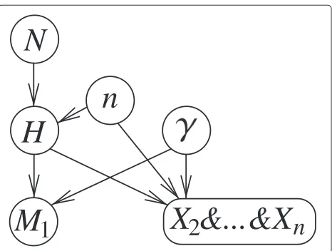
Figure 5 represents a generalization of the Bayesian net-work shown in Figure 2 to situations in which the size of the database n is greater than 2 (withn ≤ N). The following modifications are introduced:
1. The size of a database is modeled explicitly in terms of a distinct nodenwith exemplary numerical states2, 10, 100(other database sizesn≤Nmay obviously be chosen).
2. The nodeHhas three states.H1represents the proposition according to which the suspect is the source of the crime stain. The proposition according to which one of the individuals2, ...,nis the source of the crime stain is represented by the stateH2n. The third state isHn+1N. It represents the proposition that one of theN−nindividuals outside the database is the source of the crime stain. Assuming again prior
probabilities of1/Nfor each of theNindividuals, the following node probabilities are specified:
Pr(H1)=1/N, Pr(H2N)=n−1/N,
Pr(Hn+1N)=(N−n)/N.
n
N
M
H
1
n
X &...&X
2
Figure 5Bayesian network for a search of a database of size
n>2.Structure of a Bayesian network for evaluating a
correspondence (M1) between the profile of a crime stain and that of a sample from a suspect when the suspect is on a database along withn−1 other individuals. The size of the population of potential offenders isNwheren(withn≤N) of them are on a database. The nodeHhas three states: ‘the suspect is the source of the crime stain’ (H1), ‘one of then−1 other individuals in the database is the source of the crime stain’ (H2n), and ‘the source of the crime stain is among theN−nindividuals outside the database’ (Hn+1N). The
3. The probability table for the nodeM1, the
proposition according to which the suspect’s profile corresponds, contains the following values:
Pr(M1|Hi,γ )=
1, i=1,
γ, i=1 .
4. The nodeX2&...&Xnrepresents the proposition according to which then−1individuals in the database other than the suspect have profiles that do not correspond to that of the crime stain. The node probability table contains the following assignments:
Pr(X2&...&Xn|Hi,n,γ )=
⎧ ⎪ ⎨ ⎪ ⎩
(1−γ )n−1, i=1, 0, i=2, ...,n, (1−γ )n−1, i=n+1, ...,N.
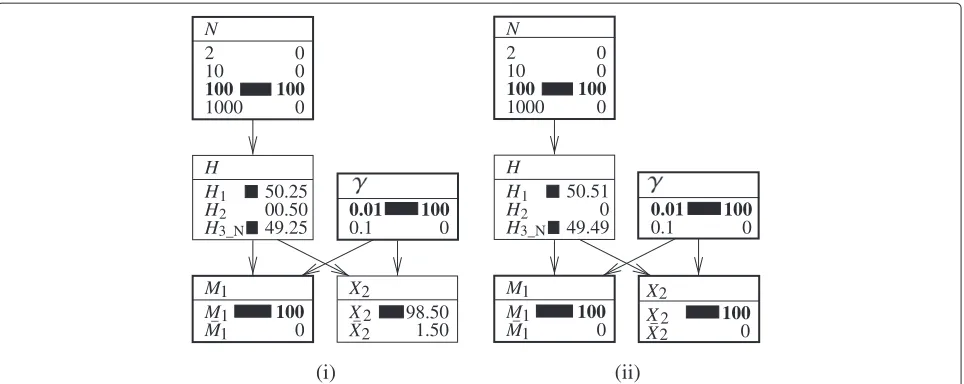
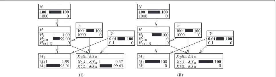
Figure 6 provides a graphical illustration of the Bayesian network described in this section. In Figure 6i, the initial situation is one with the database of sizen =100, which equals the size of the population of potential offenders, N. As a definitional implication of this, the prior proba-bility for the suspect being the source of the crime stain is 1/N = 0.01 and that for then−1 individuals in the database other than the suspect is given by the comple-ment,(N−1)/N = 0.99. Because there are no potential sources outside the database, the initial probability of the propositionHn+1N is zero. Figure 6ii illustrates the effect
of learning that none of the individuals 2, ...,nhas a profile matching that of the crime stain. This has two logical consequences. Firstly, the propositionH2nmust be false.
Secondly, probability must thus be ‘redistributed’ among the remaining ‘possible’ propositions. The propositionH1
is the only one of this kind. It thus assumes probability 1.
A Bayesian network guided derivation of the ‘database search likelihood ratio’
So far in this paper, the discussion has concentrated on the evaluation of database search results given multiple propositions. In fact, each individualiof the population of potential sourcesi(of sizeN) was considered in terms of a distinct propositionHi. In order to facilitate the
pre-sentation, theipropositions have been grouped:H1refers
to the suspect only,H2n refers to then− 1 individuals
in the database other than the suspect, andHn+1N refers
to the individuals outside the database. The consideration of multiple proposition has directed the analysis to poste-rior probabilities of the single propositionH1(that is, ‘the
suspect is the source of the crime stain’). Likelihood ratios have not primarily been addressed here because they com-pare propositions in pairs. In the analysis of scientific evi-dence, likelihood ratios play an important role, however, so that it is desirable to include them in this discussion.
A general likelihood ratio procedure for comparing more than two propositions has been described, for exam-ple, by [34]. It will be used hereafter to derive a likeli-hood ratio with reference to the Bayesian network shown in Figure 5. It starts by grouping the propositions H2n
andHn+1Nas the propositionH¯1. It represents the
propo-sition according to which the crime stain comes from some other person than the suspect (either from some other person in the database or from someone outside the database). This proposition forms a pair along withH1,
that is, ‘the suspect is the source of the crime stain’. Following considerations outlined in the section ‘Bayesian network for a search of a database of size n > 2’, letX2&...&Xndenote the evidence that none of then−1
individuals in the database has a DNA profile correspond-ing to that of the crime stain. Assumcorrespond-ing that the prior probabilities for each of the propositionsHican be given,
the ratio of the probability of the the evidence given each
0
H H H1
2_n n+1_N
H
1.00 99.00 0
2
_ 2
1 1 1
100
M M M
X &...&Xn
X &...&Xnn _________2
2
0.01 0.1 1000
X &...&X
0 0
100
H H H1
2_n n+1_N
H
0 100 0
_
2
(i)
1 1 1
98.01 1.99
M M M
X &...&Xn
X &...&Xnn
0.37 99.63
X &...&X_________
2
0 100 1000
100
N
n
1000 100 100
0 0.01 0.1 1000
0 100 1000
100
N
n
1000 100 100
(ii)
of the pair of propositions H1 and H¯1, called database
likelihood ratio here (LRDB), can be evaluated as follows:
LRDB=
Pr(X2&...&Xn|H1)
Pr(X2&...&Xn| ¯H1)
= Pr(X2&...&Xn|H1){
N
i=2Pr(Hi)}
N
i=2Pr(X2&...&Xn|Hi)Pr(Hi)
. (14)
The denominator of this expression can be extended as follows:
n
i=2
Pr(X2&...&Xn|Hi)Pr(Hi)
+
N
i=n+1
Pr(X2&...&Xn|Hi)Pr(Hi).
The first part of this sum cancels because the likelihoods for then−1 individuals in the database, other than the suspect, are zero. The likelihood ratio, Equation 14, thus reduces to the following:
LRDB=
Pr(X2&...&Xn|H1)
Pr(X2&...&Xn| ¯H1)
= Pr(X2&...&Xn|H1){Ni=2Pr(Hi)}
N
i=n+1Pr(X2&...&Xn|Hi)Pr(Hi)
. (15)
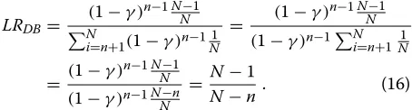
The likelihood for the suspect and the individuals out-side the database is(1−γ )n−1. The prior probability for each individualito be the source of the crime stain is, as it was assumed throughout this paper, 1/N. Equation 15 can thus be rewritten as follows:
LRDB=
(1−γ )n−1NN−1
N
i=n+1(1−γ )n−1 1N
= (1−γ )n−1NN−1 (1−γ )n−1N
i=n+1N1
= (1−γ )n−1N−
1 N (1−γ )n−1N−n
N
= N−1
N−n. (16)
According to this result, the likelihood ratio is maximal when the size of the database,n, equals that of the popula-tion of potential sources,N. The logic of this result is also illustrated by the Bayesian network depicted in Figure 6ii. It shows that knowledge of X2&...&Xn implies the truth
ofH1in a setting in whichN =n. Conversely, if the
sus-pect is the only person in the database (n=1), this means that there is no information about excluded individuals. Accordingly, withn=1, the value forLRDBis one.
The Bayesian network discussed so far (Figure 5) can be adapted in order to illustrate a likelihood ratio evalu-ation. As a minor modification, it is necessary to add a summary nodeH1with two statesH1(‘the suspect is the
source of the crime stain’) and H¯1 (‘some person other
than the suspect is the source of the crime stain’). The
latter state regroups the two propositionsH2nandHn+1N
of the nodeH. The nodeH1is added as a descendant of the
nodeH. The probability table contains the logical values 0 and 1 as shown in Table 5.
This extension is shown in Figure 7. The figure on the left shows an evaluation of the numerator of the likeli-hood ratio. The nodeH1is set toH1which implies also
that that nodeHwill displayH1as ‘true’. Because the
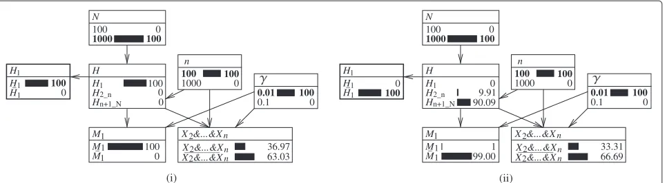
rar-ity of the characteristic γ is set to 0.01 and the size of the database n to 100, the probability that none of the othern−1 individuals in the database has a correspond-ing profile is(1−γ )n−1=0.9999 =0.3697. This value is shown in the nodeX2&...&Xn.
The evaluation of the denominator is shown in Figure 7ii. Here, the nodeH1is set toH¯1. This implies that
the stateH1 in the nodeH is zero. Accordingly,
proba-bility is redistributed proportionally among the remaining propositionsH2nandHn+1N. In fact, if the suspect is not
the source of the crime stain (that is,H¯1is true), then (a)
there is a probability of(n−1)/(N−1)=99/999=0.0991 that someone other than the suspect inside the database is the source of the crime stain, and (b) there is a prob-ability of (N −n)/(N − 1) = 900/999 = 0.9009 that someone outside the database is the source of the crime stain. These two probabilities are displayed in the nodeH. Finally, the probability that none of then−1 individuals in the database (other than the suspect) matches, given that the suspect is not the source of the crime stain, is given as follows:
Pr(X2&...&Xn| ¯H1) = Pr(X2&...&Xn|H2n)Pr(H2n| ¯H1) +Pr(X2&...&Xn|Hn+1N)Pr(Hn+1N| ¯H1) = 0×(n−1)/(N−1)
+(1−γ )n−1×(N−n)/(N−1) = 0.9999×900/999=0.3331 .
This result is obtained in the node X2&...&Xn in
Figure 7ii.
More generally, it also worth noting that the evidential value of ‘excluding’ indiviuals 2, ...,ndoes not depend on the rarity of the compared analytical characteristicγ but only on the size of the target population and the size of the database. The evidence will be stronger or weaker depend-ing on whether the database covers, respectively, a greater or a smaller proportion of the population.
Table 5 Probability table for summary nodeH1
H: H1 H2n Hn+1N
H1 1 0 0
¯
H1 0 1 1
1
n
1000
100 100
0
(ii)
X &...&Xn
X &...&Xnn
2 2
X &...&X
2
63.03 36.97 n
1000
100 100
0 0.01 0.1 0
100
_________ _
_
1 1 1
100 M
M
M 0
M M M
1 1 1
_ _________
H H H1
2_n
H
n+1_N
H
H
1000 100 N
0 100
H
1
1 1 _
100
0 0
9.91 90.09
99.00 1
0.01 0.1 0
100
X &...&Xn
X &...&Xnn
2 2
X &...&X
2
66.69 33.31
(i)
H H H1
2_n
H
0 100 0 n+1_N
H
H
1000 100 N
0 100
H 100 0 1
1
Figure 7Alternative representations of a Bayesian network for a search of a database of sizen>2.Bayesian network shown in Figure 5 with expanded representation of nodes along with an additional nodeH1with statesH1(‘the suspect is the source of the crime stain’) andH¯1(‘some person other than the suspect is the source of the crime stain (either someone else in the database or an individual outside the database)’). Both figures show a situation in which the sizenof the database equals 100 and that of the suspect population,N, equals 1,000. The rarity of the corresponding characteristic is set to 0.01.(i)Illustration of the evaluation of the numerator of the likelihood ratio for the item of
informationX2&...&Xn(that is, none of then−1 individuals in the database other than the suspect corresponds to the crime stain):H1is set to ‘true’, and the value of the numerator is shown in the nodeX2&...&Xn.(ii)An evaluation of the denominator of the likelihood ratio (that is,H¯1is set to ‘true’). Probabilities are shown in percentages.
Conclusions
Logically compelling argument has been presented in sci-entific literature in support of the argument that excluding individuals in a database represents evidence that tends to strengthen the case against a matching suspect [18,35]. It is widely conceded, however, that the associated mathe-matics is not easy to explain, in particular to lay persons, and even so in trial proceedings. It is therefore desirable that, at least among forensic scientists and legal profes-sionals, there is a common and agreed understanding of the proofs and logic that support the prevalent scientific opinion in this area.
However, within the scientific community, this seems to be a difficult endeavor. This is illustrated, for example, by the critical debates that have at some point accompanied the discussion of settings in which a suspect was selected through a database search, as is illustrated by [14,36]. In some parts of the forensic community, opinions cur-rently persist according to which a database search should ‘weaken’ a case against the suspect. A recent example for this is a recommendation issued by the German Stain Commission [33]. That document falls for the known mis-conception that it should be of concern that one is looking for individuals that possess a profile that corresponds to the crime stain. This is motivated by the intuitively appeal-ing but logically unfounded argument that (1) it is unsur-prising to see that the suspect that is found as a result of a database search will present the target profile, and (2) therefore, the corresponding crime stain profile ought to be of little or reduced evidential value. It seems that such opinion is influenced by asking questions of the follow-ing kind: ‘What are the chances of findfollow-ing an individual that has the crime stain genotype if one is searching for individuals who could possess that genotype (for example,
by searching a database)?’ However, this is not a very help-ful question because it does not serve well the needs of the recipients of expert information. They rather seek infor-mation regarding a question of the following kind: ‘Given that a person was found with a profile that corresponds to that of a crime stain, what is the strength of the evidence against this suspect?’
As mentioned above, the principal routes of logical anal-ysis lead to the conclusion that the case against a matching suspect is strengthened when excluding other potential donors. This may be pointed out either through analy-ses of the posterior probability of the proposition that the suspect is the source of the crime stain or through a likelihood ratio analysis. The rigor of the analyses put forward in literature is also paired with convincing impli-cations in limiting cases, that is, when all potential sources are excluded, then the procedures indicate that the only matching suspect must be the crime stain donor. When no individuals other than the suspect are investigated, then the case against the suspect reduces to the evaluation of a one-stain one-offender case. Such a case may, within some general assumptions, be assessed in terms of the inverse of the random match probability [16].
inferential procedures have common underlying patterns of inference. Therefore, a Bayesian network approach is not only helpful for examining the logic within a given inferential procedure, but is also valuable for checking the coherence between different inferential approaches (here: the relationship between the island problem and the database search issue).
More generally, starting with the island problem is help-ful because it is well posed. It is instructive to point out the rationale of the argument in a ‘simple world’ context. This can favor the understanding of the main principle of the argument without possible distraction due to partic-ular numerical settings. The inherent reason behind the searching among islanders is that any individual found to have a profile other than that of the crime stain is excluded−under the assumption of absence of laboratory error−as a potential source. The pool of potential donors thus becomes smaller with the corollary that the suspicion against each remaining potential source must increase. Stated otherwise, probability is to be redistributed among fewer candidates.
The Bayesian network approach discussed in this paper provides a clear illustration for this. In Figure 8, a case with a population size N = 1, 000 and n = 100 is considered, along with an analytical characteristic which occurs with probability γ = 0.01. Knowing that the individuals 2, ...,n do not correspond to the crime stain sets the proposition H2n, that one of the n − 1
indi-viduals of the database is the source of the crime stain, to zero. Accordingly, probability must be redistributed among the propositions H1 (‘the suspect is the source
of the crime stain’) and Hn+1N (‘the true source of the
crime stain is outside the database’). It then becomes a question to know how this ought to be operated. If one assumes that, initially, each individual i had the
same probability of being the source of the crime stain, then Pr(Hi) = 1/N (for i = 0, 1, ...,N). Next, if one
excludes the individuals i = 2, ...,n, then the poste-rior probability for the remaining individuals must reflect ‘a proportional increase’. For example, if the proposi-tion for the suspect initially had a probability of 1/N, it has 1/(N−n+1) after excluding then−1 individuals in the database (other than the suspect). This is shown in the Bayesian network in Figure 8 where, after consider-ation of the evidenceX2&...&Xn, the propositionH1has
the probability 1/(N−n+1) = 0.00111 and the propo-sitionHn+1N has the probability(N−n)/(N−n+1)=
0.99889.
The graphical display in the proposed Bayesian network is particularly compelling. If probability from one proposi-tion (here:H2n) is taken, then it must well ‘go’ somewhere
because, on the whole, the condition Ni=1Pr(Hi) = 1
must remain satisfied. It is not conceivable that probability is transferred exclusively toHn+1N, as suggested by
pro-ponents of a decreasing probative value due to a database search. The reason for this is that with increasing database sizen, the number of distinct propositions (that is, indi-viduals) subsumed underHn+1N decreases. By all logic,
the propositionH1must thus be reinforced.
A Bayesian network approach was pursued in this paper because it has the advantage of offering a concise repre-sentation and description of (1) the various components (variables and probability assignments) that make up a given inferential procedure as well as (2) their relation-ships. From a purely descriptive point of view, the general Bayesian network proposed here in Figure 5 allows one to point out the following aspects:
1. The size of the databasen and the size N of the population of potential sources can be used to define
0
M M M
1 1 1
_ _________
H H H1
2_n H
n+1_N H
H
1000
100 N
0
100
H 1
1 1 _
99.89
0.01
0.1 0
100
X &...&Xn
X &...&Xnn
2 2
X &...&X
2
99.89 0.110
98.89
1.11 100
0 0.11
n
1000
100 100