Efficient Estimator for Population Variance Using Auxiliary Variable

Efficient Estimator for Population Variance Using

Auxiliary Variable

Subhash Kumar Yadav1_{, Sheela Misra}2_{, S. S. Mishra}1,*

1_{Department of Mathematics and Statistics (A Centre of Excellence), Dr. RML Avadh University, Faizabad, U.P., India} 2_{Department of Statistics, University of Lucknow, Lucknow, U.P., India}

Abstract

Population variance is one of the important measures of dispersion. For example one is interested in knowing the estimate of variance of a particular crop, blood pressure, temperature etc. This paper deals with the estimation of population variance using auxiliary information under simple random sampling scheme. In the present paper, we have proposed an improved estimator through well known kappa technique using Yadav et al (2014) paper. The large sample properties of the estimator have been studied up to the first order of approximation that is its bias and mean square error have been obtained up to the first order of approximation. The optimum value of the characterizing scalar kappa has been obtained and for this optimum value of the kappa the minimum mean squared error has been obtained. A comparison has been made with the existing estimators of population variance using secondary data. An improvement of the proposed estimator has been shown over all existing mentioned estimators as it has lesser mean square error as compared to other estimators.

Keywords

Ratio estimator, Quartiles, Bias, Mean squared error, Efficiency

1. Introduction

In the theory of survey sampling, the auxiliary information plays paramount role in developing and searching improved estimators of population parameters of the study variable. The auxiliary information is used at both the stages of designing and estimation. Here we have used this information at estimation stage only. The auxiliary variable (X) and the main variable (Y) under study are highly closely related with each other. When there is a close positive association between the study variable and the auxiliary variable and the line of regression of the study variable Y on the auxiliary variable X passes through origin, then the ratio type estimator is used for improvement over the parameters of the population under consideration. On the other hand the product type estimators are used for improved estimation of parameters when the auxiliary variable X and the study variable Y have negative correlation between them. While the regression type estimators are used for the improved estimation of population parameters, when the line of regression does not pass through the origin.

Let the population under investigation is finite and it consists of N distinct and identifiable units. Let

( , ),

x y i

_{i i}

=

1,2,...,

n

be a random sample of size n from above bivariate population (X, Y) of size N using a

* Corresponding author:

[email protected] (S. S. Mishra) Published online at http://journal.sapub.org/ajor

Copyright © 2016 Scientific & Academic Publishing. All Rights Reserved

SRSWOR scheme. Let

X

and

Y

respectively are the population means of the auxiliary and the study variables, and let

x

and

y

are the corresponding sample means which are unbiased estimators of population means

X

_and

Y

respectively. Let

ρ

denote the correlation coefficient between the variables X and Y and

Q

_r is the inter-quartile range of the auxiliary variable X. In this manuscript, we have proposed an improved ratio type estimator of population variance of study variable by suitably using the correlation coefficient

ρ

_{between the two variables and}

Q

_r , inter-quartile range of the auxiliary variable X. Further we assume that a reliable estimate of the correlation coefficient

ρ

_{is available in advance from pilot surveys etc.}

2. Variance Estimators in Literature

The sample variance is the most appropriate estimator of population variance and is given by:

2

0 y

t

=

s

, (2.1) This estimator of population variance is unbiased, and it has the variance up to the first degree of approximation as:

)

1

(

)

(

t

0

=

γ

S

y4

λ

40

−

2 2 2x R y x

S

t

s

s





= 







, (2.3)

where

2 2

1

1

₍

₎

1

n

y i

i

s

y y

n

=

=

−

−

∑

, 2 11 ₁( )2

n

x i

i

s x x

n

= −

−

∑

₌ , 2 ₁ 2

1 _{( )}

1

N

x i

i

S X X

N = = − −

∑

, 1 1 N i i X X N ₌ =

∑

, 1 1 N i i Y Y N ₌ =

∑

, 1

1

n i i

x

x

n

₌

=

∑

, 1

1

n i i

y

y

n

=

=

∑

.

The first order of approximations for the Bias and Mean Square Error (MSE) respectively are given by

)]

1

(

)

1

[(

)

(

t

R

=

γ

S

y2

λ

04

−

−

λ

22

−

B

, (2.4)

)]

1

(

2

)

1

(

)

1

[(

)

(

t

R

=

γ

S

4y

λ

40

−

+

λ

04

−

−

λ

22

−

MSE

, (2.5)

where

2 2 20 02

rs rs r s

µ

λ

µ µ

=

,

1

1 _{( ) ( )}

1

N _{r s}

rs i i

i Y Y X X

N

µ

=

= − −

−

∑

,

n

f

−

=

1

γ

and

f

n

N

=

.

Several authors proposed different estimators by utilizing auxiliary information in different forms. They used it in the form of different parameters of auxiliary variable for estimating the population variance of the main variable under study. Some of them from the literature are as follows,

Upadhyaya and Singh (1999) utilized coefficient of kurtosis

β

_2(x) of auxiliary variable and proposed the following estimator of population variance as,

















+

+

=

) ( 2 2 ) ( 2 2 2 2 1

ˆ

x x x x y

_s

S

s

S

β

β

(2.6)

The bias and Mean Squared Error of above estimator up to the first order of approximations respectively are,

[

(

1

)

(

1

)

]

)

ˆ

(

2 2 _{1 1 04 22} 1

=

γ

S

R

R

λ

−

−

λ

−

S

B

y

[

(

1

)

(

1

)

2

(

1

)

]

)

ˆ

(

2 _{04 1 22}

1 40

4 2

1

=

γ

S

λ

−

+

R

λ

−

−

R

λ

−

S

MSE

y (2.7)

Where, ) ( 2 2 2 1 x x x

S

S

R

_β

+

=

Kadilar and Cingi (2006) proposed the following estimators using different parameters of auxiliary information as,













+

+

=

x x x x y

_s

_C

C

S

s

S

2 2 ₂2

2

ˆ

,

















+

+

=

x x x x x x y

C

s

C

S

s

S

) ( 2 2 ) ( 2 2 2 2 3

ˆ

β

β

,

















+

+

=

) ( 2 2 ) ( 2 2 2 2 4

ˆ

x x x x x x y

C

s

C

S

s

S

β

β

The bias and Mean Squared Error of above estimators up to the first order of approximations respectively are,

[

(

1

)

(

1

)

]

)

ˆ

(

2

₌

_γ

2

_λ

₀₄

₋

₋

_λ

₂₂

₋

i i y i

S

R

R

S

B

[

(

1

)

(

1

)

2

(

1

)

]

)

ˆ

(

2 _{04 22}

40 4

2

₌

_γ

_λ

₋

₊

_λ

₋

₋

_λ

₋

i i

y

i

S

R

R

S

MSE

i

=

2

,

3

,

4

(2.8)

Where, x x x

C

S

S

R

+

=

₂ 2

2 , x x x x x

C

S

S

R

+

=

) ( 2 2 ) ( 2 2 3

_β

β

, ) ( 2 2 2 4 x x x x x

C

S

C

S

R

β

+

=













+

+

=

1 2 1 2 2 2 5

ˆ

Q

s

Q

S

s

S

x x

y ,













+

+

=

3 2 3 2 2 2 6

ˆ

Q

s

Q

S

s

S

x x

y , 

     + + = r x r x y S_{s Q}Q

s S2 2 ₂2

7 ˆ ,

_











+

+

=

d x d x y

S

_s

_Q

Q

s

S

2 2 ₂2

8

ˆ

_,

_











+

+

=

a x a x y

S

_s

_Q

Q

s

S

2 2 ₂2

9

ˆ

The expressions for the bias and Mean Squared Error of above estimators up to the first order of approximations respectively are,

[

(

1

)

(

1

)

]

)

ˆ

(

S

i2

=

γ

S

y2

R

i

R

i

λ

04

−

−

λ

22

−

B

[

(

1

)

(

1

)

2

(

1

)

]

)

ˆ

(

2 _{04 22}

40 4

2

₌

_γ

_λ

₋

₊

_λ

₋

₋

_λ

₋

i i

y

i

S

R

R

S

MSE

i

=

5

,

6

,

7

,

8

,

9

(2.9) Where,

1 2

2

5

_S

_Q

S

R

x x

+

=

, 3 2 2

6

_S

_Q

S

R

x x

+

=

, r x x

Q

S

S

R

+

=

₂ 2

7 , d x x

Q

S

S

R

+

=

₂ 2

8 , a x x

Q

S

S

R

+

=

₂ 2 9

Where

Q

_i

( 1,2,3)

i

=

are the quartiles, the three points dividing the whole distribution into four equal parts. Further the functions of quartiles are, the inter quartile range,

Q Q Q

_r

=

₃

−

₁, the semi-quartile range 3 1

2

d Q Q

Q = − and the quartile

average 3 1

2

a

Q Q

Q

=

+

.

Khan and Shabbir (2013) proposed the following estimator using correlation coefficient and the third quartile of the auxiliary variable as,













+

+

=

3 2 3 2 2 2 10

ˆ

Q

s

Q

S

s

S

x x y

_ρ

ρ

The expressions for the bias and Mean Squared Error of the estimator up to the first order of approximations respectively are,

[

(

1

)

(

1

)

]

)

ˆ

(

2 2 _{10 10 04 22} 10

=

γ

S

R

R

λ

−

−

λ

−

S

B

y

[

(

1

)

(

1

)

2

(

1

)

]

)

ˆ

(

2 _{04 10 22}

10 40

4 2

10

=

γ

S

λ

−

+

R

λ

−

−

R

λ

−

S

MSE

y (2.10)

Where,

3 2

2

10

_S

S

_Q

R

x x

+

=

ρ

ρ

Yadav et al. (2014), utilizing the correlation coefficient of the inter-quartile range of auxiliary variable proposed the following estimator as,













+

+

=

r x r x y

S

_s

_Q

Q

s

S

2 2 ₂2

_ρ

ρ

11

ˆ

The bias and Mean Squared Error of the above estimator up to the first order of approximations respectively are,

[

(

1

)

(

1

)

]

)

ˆ

(

2 2 _{11 11 04 22} 11

=

γ

S

R

R

λ

−

−

λ

−

S

B

y

[

(

1

)

(

1

)

2

(

1

)

]

)

ˆ

(

2 _{04 11 22}

11 40

4 2

11

=

γ

S

λ

−

+

R

λ

−

−

R

λ

−

S

MSE

y (2.11)

Where, r x x

Q

S

S

R

+

=

ρ

ρ

2 2 11 .

3. Proposed Estimator













+

+

=

r x

r x y

S

_s

_Q

Q

s

t

ρ

ρ

κ

2 ₂2 _{, (3.1)}

where

κ

is a characterizing scalar to be determined such that the MSE of the proposed estimator

t

is minimized. To obtain the bias and Mean squared error of the proposed estimator, we wish to define

(

₀

)

2 2

_S

₁

_e

s

y

=

y

+

and

s

x2

=

S

x2

(

1

+

e

1

)

such that

E

( )

e

i

=

0

for

(

i

=

0,1)

and

( )

02

1

(

40

−

1

)

−

=

λ

n

f

e

E

,

( )

2

1

(

₀₄

1

)

0

−

−

=

λ

n

f

e

E

,

(

_{0 1}

)

=

1

−

(

λ

₂₂

−

1

)

n

f

e

e

E

.

The proposed estimator

t

can be written in terms of

ε

_i’s (

i

=

0

,

1

), as 1 1 11 0

2

₍

₁

₊

₎₍

₁

₊

₎

−

=

S

e

R

e

t

κ

y

Expanding the right hand side of above equation and considering the terms in

ε

_i’s up to the first degree of approximation, we get:

)

1

(

2

1 2 11 1 0 11 1 11 0

2

_e

_R

_e

_R

_e

_e

_R

_e

S

t

=

κ

_y

+

−

−

+

After subtracting the population variance

S

2_y of study variable on both the sides of above equation, we have, 2

2 1 2 11 1 0 11 1 11 0 2

2

₍

₁

₎

y y

y

S

e

R

e

R

e

e

R

e

S

S

t

−

=

κ

+

−

−

+

−

(3.2) The bias of proposed estimator

t

is obtained by taking expectations on both sides of (3.2) and putting the values of different expectations, as:

)

1

(

)]

1

(

)

1

(

[

)

(

2

22 11 04

2 11

2

₋

₋

₋

₊

₋

=

λκ

S

_y

R

λ

R

λ

S

_y

κ

t

B

(3.3)

where

(1

f

)

n

λ

=

−

.

The mean squared error of the proposed estimator

t

is obtained by squaring both sides of (3.2), simplifying and taking expectation on both sides, up to the first order of approximation as,

]

)

1

(

)

1

(

)

2

(

2

)

1

(

)

2

3

(

)

1

(

[

)

(

2

22 11 2

04 2 11 2

40 2

4

₋

₊

₋

₋

₋

₋

₋

₊

₋

=

S

κ

λ

λ

κ

κ

R

λ

λ

κ

κ

R

λ

λ

κ

t

MSE

y (3.4)

)

(

t

MSE

is minimum for,

B

A

=

κ

(3.5)

where,

)

1

(

)

1

(

1

+

112 04

−

−

11 22

−

=

R

λ

λ

R

λ

λ

A

and

)

1

(

4

)

1

(

3

)

1

(

1

2 _{04 11 22}

11

40

−

+

−

−

−

+

=

λ

λ

R

λ

λ

R

λ

λ

B

The minimum MSE of the estimator,

t

, for this optimum value of

κ

, is:













−

=

B

A

S

t

MSE

y

2 4

min

(

)

1

(3.6)

4. Efficiency Comparison













−

−

−

=

−

(

)

1

(

1

)

)

(

40

2 2

0

min

t

V

t

S

A

_B

λ

λ

MSE

y

<

0,

if

(

40

1

)

1

2

>

−

+

λ

λ

B

A

_(4.1)

The proposed estimator in (3.1) will perform better than the estimator (2.3), under the condition if:

{

}

_











−

−

−

+

−

−

−

=

−

(

)

1

(

1

)

(

1

)

2

(

1

)

)

(

40 04 22

2 2

min

t

MSE

t

S

A

_B

λ

λ

λ

λ

MSE

_{R y}

<

0,

if

{

(

40

1

)

(

04

1

)

2

(

22

1

)

}

1

2

>

−

−

−

+

−

+

λ

λ

λ

λ

B

A

_(4.2)

The proposed estimator

t

has more efficiency as compared to all other estimators

ˆ

2

i

S

(i=1,2,...,11) mentioned in this manuscript under the condition if:

)

ˆ

(

)

(

2

min

t

MSE

S

i

MSE

−

{

}

_











−

−

−

+

−

−

−

=

1

(

40

1

)

2

(

04

1

)

2

(

22

1

)

2

2

_λ

_λ

_λ

_λ

i i

y

A

_B

R

R

S

<

0,

(

i

=

1

,

2

,

...,

11

)

if

{

(

₄₀

1

)

2

(

₀₄

1

)

2

(

₂₂

1

)

}

1

2

>

−

−

−

+

−

+

λ

λ

R

_i

λ

R

_i

λ

B

A

_{, (4.3)}

5. Numerical Illustration

Following populations have been considered to examine the performances of different estimators of population variance,

Population I: Italian bureau for the environment protection-APAT Waste 2004

Y: Total amount (tons) of recyclable-waste collection in Italy in 2003.

X: Total amount (tons) of recyclable-waste collection in Italy in 2002.

103

=

N

,

n

=

40

,

Y

=

626

.

2123

, X =557.1909,

9936

.

0

=

ρ

,

S

_y

=

913

.

5498

,

C

_y

=

1

.

4588

,

1117

.

818

=

x

S

,

C

_x

=

1

.

4683

,

λ

₀₄

=

37

.

3216

,

1279

.

37

40

=

λ

,

λ

₂₂

=

37

.

2055

,

Q

₁

=

142

.

9950

,

6250

.

665

3

=

Q

,

Q

_r

=

522

.

6300

,

Q

_d

=

261

.

3150

,

3100

.

404

=

a

Q

.

Population II: Italian bureau for the environment protection-APAT Waste 2004

Y: Total amount (tons) of recyclable-waste collection in Italy in 2003.

X: Number of inhabitants in 2003.

103

=

N

,

n

=

40

,

Y

=

62

.

6212

, X =556.5541,

7298

.

0

=

ρ

,

S

_y

=

91

.

3549

,

C

_y

=

1

.

4588

,

1643

.

610

=

x

S

,

C

_x

=

1

.

0963

,

λ

04

=

17

.

8738

,

1279

.

37

40

=

λ

,

λ

₂₂

=

17

.

2220

,

Q

₁

=

259

.

3830

,

0235

.

628

3

=

Q

, Q_r =368.6405, Q_d =184.3293,

7033 . 443

= a

Q .

Population III: Murthy (1967) Y: Output for 80 factories in a region. X: Fixed capital.

80

=

N

,

n

=

20

,

Y

=

51

.

8264

,

X

=

11

.

2646

,

9413

.

0

=

ρ

,

S

_y

=

18

.

3549

,

C

_y

=

0

.

3542

,

4563

.

8

=

x

S

,

C

_x

=

0

.

7507

,

λ

₀₄

=

2

.

8664

,

2667

.

2

40

=

λ

,

λ

₂₂

=

2

.

2209

,

Q

₁

=

5

.

1500

,

975

.

16

3

=

Q

,

Q

_r

=

11

.

825

,

Q

_d

=

5

.

9125

,

0625

.

11

=

a

Q

.

Population IV: Singh and Cahudhary

The population consists of 70 wheat farms in 70 villages in certain region of India and the variables under considerations are defined as:

Y = area under wheat crop (in acres) during 1974, X = area under wheat crop (in acres) during 1973,

70

=

N

,

n

=

25

,

Y

=

96

.

7000

,

X

=

175

.

2671

,

7293

.

0

=

ρ

,

S

y

=

60

.

7140

,

C

y

=

0

.

6254

,

8572

.

140

=

x

S

,

C

_x

=

0

.

8037

,

λ

₀₄

=

7

.

0952

,

7596

.

4

40

=

λ

,

λ

₂₂

=

4

.

6038

,

Q

₁

=

80

.

1500

,

0250 . 225

3 =

Q ,

Q

r

=

144

.

8750

,

Q

d

=

72

.

4375

,

5875

.

152

=

a

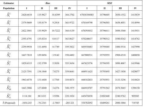
Table 1. Comparison of Bias and Mean square error of different estimators

Estimator Bias MSE

Population I II III IV I II III IV

2 1

ˆ

S

2420.6810 135.9827 10.4399 364.3702 67038384403 35796605 3850.1552 1415839 2

2

ˆ

S

2379.9609 135.8179 9.2918 363.9722 670169790 35796503 3658.4051 1414994 2

3

ˆ

S

2422.3041 135.9929 10.7222 364.4139 670393032 35796611 3898.5560 1415931

2 4

ˆ

S

2393.4791 135.8334 8.8117 363.8627 670240637 35796512 3580.8342 1414762 2

5

ˆ

S

2259.9938 133.4494 8.1749 359.3822 669558483 35795045 3480.5516 1427990

2 6

ˆ

S

1667.7818 129.8456 3.9142 350.4482 667000531 35792955 2908.6518 1408858

2 7

ˆ

S

1829.6315 132.3799 5.5038 355.3634 667623576 35794395 3098.4067 1419946

2 8

ˆ

S

2125.7591 134.1848 7.8275 359.8641 668911625 35795495 3427.1850 1429077

2 9

ˆ

S

1963.6570 131.6458 5.7705 354.8875 668182833 35793951 3133.3256 1418424

2 10

ˆ

S

1663.3086 127.6040 3.6276 348.1975 666910707 35791562 2878.5603 1398150

2 11

ˆ

S

1114.184 80.1433 3.9396 228.1034 645476858 21882440 2240.9762 905945

t

(Proposed) -1034.243 -76.2341 -2.7865 -203.321 534782692 16409261 2080.1004 718745

6. Results and Conclusions

This paper deals with the estimation of population variance using improved ratio type estimator. An efficient estimator of population variance using coefficient of correlation and the inter quartile range of the auxiliary variable has been proposed. Up to the first degree of approximation, the expressions for the bias and mean square error of the proposed estimator have been obtained. The optimum value of the characterizing scalar kappa, which minimizes the mean squared error of the proposed estimator, is also obtained. Further the minimum value of the mean square error for this optimum value of kappa has also been obtained. It has been proved theoretically as well as empirically that the proposed estimator performs much better than all of the other mentioned estimators of population variance in the sense of having lesser Bias and MSE. It is of worth to be mentioned that the knowledge regarding the correlation coefficient

ρ

should be available in advance. This knowledge of correlation coefficient is either available in advance (generally) or it is obtained from prior studies like pilot surveys etc. In case if we do not have prior knowledge of correlation coefficient, then it in the expression of estimator is replaced by its estimate and there is no effect on the mean squared error the estimator. Therefore it is strongly recommended that the proposed estimator should be

preferred over the estimators mentioned in this manuscript for the estimation of population variance under simple random sampling scheme.

ACKNOWLEDGEMENTS

The authors are very much thankful to the editor in chief of AJOR and the anonymous learned referees for critically examining the manuscript and giving the valuable suggestions for further improvement in the earlier draft.

REFERENCES

[1] Isaki, C, T., Variance estimation using auxiliary information,

Journal of American Statistical Association, 78, 117- 123 (1983).

[2] Kadilar, C. and Cingi, H., Improvement in variance estimation using auxiliary information, Hacettepe Journal of mathematics and Statistics, 35, 111-15 (2006).

[4] Khan, M. and Shabbir, J., A Ratio Type Estimator for the Estimation of Population Variance using Quartiles of an Auxiliary Variable, Journal of Statistics Applications & Probability, 2, 3, 319-325 (2013).

[5] Murthy, M. N., Sampling Theory and Methods, Statistical Publishing Society Calcutta, India, (1967).

[6] Singh, D. and Chaudhary, F. S., Theory and analysis of sample survey designs, New-Age International Publisher, (1986).

[7] Subramani, J. and Kumarapandiyan, G., Variance estimation using quartiles and their functions of an auxiliary variable,

International Journal of Statistics and Applications, 2, 67-72 (2012).

[8] Upadhyaya, L. N. and Singh, H. P., Use of auxiliary information in the estimation of population variance, mathematical forum, 4, 33-36 (1983).

[9] http://www.osservatorionalerifiuti.it/ElencoDocPub.asp?A_ TipoDoc=6.