Galley
Pro
of
Vol. 8, No. 2, (2018), pp 95–117 DOI:10.22067/ijnao.v8i2.60778
Discrete collocation method for
Volterra type weakly singular integral
equations with logarithmic kernels
P. Mokhtary∗
Abstract
An efficient discrete collocation method for solving Volterra type weakly singular integral equations with logarithmic kernels is investigated. One of features of these equations is that, in general the first derivative of solution behaves like as a logarithmic function, which is not continuous at the origin. In this paper, to make a compatible approximate solution with the exact ones, we introduce a new collocation approach, which applies the M¨ untz-logarithmic polynomials(M¨untz polynomials with logarithmic terms) as basis functions. Moreover, since implementation of this technique leads to integrals with logarithmic singularities that are often difficult to solve numerically, we apply a suitable quadrature method that allows the exact evaluation of inte-grals of polynomials with logarithmic weights. To this end, we first remind the well-known Jacobi–Gauss quadrature and then extend it to integrals with logarithmic weights. Convergence analysis of the proposed scheme are pre-sented, and some numerical results are illustrated to demonstrate the effi-ciency and accuracy of the proposed method.
Keywords: Discrete collocation method; M¨untz-logarithmic polynomials; Quadrature method; Volterra type weakly singular integral equations with logarithmic kernels.
1 Introduction
In this paper, we develop an approximate approach to obtain the numerical solution of the following Volterra type weakly singular integral equation with logarithmic kernel
∗Corresponding author
Received 5 December 2016; revised 16 May 2018; accepted 13 June 2018 P. Mokhtary
Department of Mathematics, Faculty of basic Sciences, Sahand University of Technology, Tabriz, Iran. e-mail: [email protected] [email protected]
Galley
Pro
of
y(x) =g(x)+
x
∫
0
ln (x−t)K(x, t)y(t)dt, x∈Ω = [0,1], 0≤t≤x≤1, (1) where the continuous functions g(x) and K(x, t) are given andy(x) is the unknown solution. Such kinds of equations arise from solution of Dirichlet’s problem for the Laplace equation in two dimensions in terms of a single-layer logarithmic potential [24], solution of the reduced wave equation in two di-mensions using an integral equation with a kernel, which can be expressed as a Hankel function of order zero that this kernel, has also a logarithmic singularity [25], investigation of electrostatic and low frequency electromag-netic problems [15], methods of computing the conformal mapping of a given domain [28], solution of electromagnetic scattering problems( [2], [16]), deter-mination of propagation of acoustical and elastical waves( [5], [6]), boundary value problems of plane elasticity theory for regions with a defect [13], prob-lems of diffraction by thin screens [12] and so on.
Weakly singular integral equations with logarithmic kernels are usually difficult to solve analytically; so it is necessary to provide reliable numerical techniques. There are several approximate methods proposed to obtain the numerical solution of these types of equations, which we refer to some of them. In [4], authors designed a computational meshless discrete Galerkin method to solve the second kind Fredholm integral equations with logarithmic kernels. In [17], authors developed a collocation method for the numerical solution of a special integro-differential equation with logarithmic kernel using airfoil polynomials of the first kind. A collocation method based on the periodic splines was introduced in [11] to solve some logarithmic kernel integral equa-tions on open arcs. In [29], authors studied a special integral equation with logarithmic kernel and solved it using product integration method. In [14], a piecewise Chebyshev expansion was considered to solve Volterra integral equations with logarithmic singularities in their kernels. The properties of the integro-differential equations of the convolution on a finite interval with kernel having a logarithmic singularity were studied in [3]. In [10], authors investigated two numerical approaches by means of an analytical integration in the vicinity of the singular point and extraction of the singular part. A Gauss type quadrature method with a logarithmic weight function was ex-tended to evaluate of the Cauchy type integral equations with logarithmic kernels in [30].
Galley
Pro
of
polynomials [18]. Since in the implementation procedure, integrals with log-arithmic singularities are observed to highly accurate evaluation of them, we use a generalized Gauss type quadrature with logarithmic weight function that calculates exactly integrals of polynomials [7].The reminder of this paper is organized as follows. In the next section we present the required preliminaries for our subsequent development. Here, we introduce the M¨untz-logarithmic polynomials as well as the generalized Gauss quadrature method for the integrals with logarithmic weight functions. In Section 3, we explain the application of the discrete collocation method using M¨untz-logarithmic polynomials to approximate the solution of (1). In Section 4, we provide a reliable convergence analysis for the proposed algorithm that justifies theL2−norm of the error function tends to zero as the approximation
degree tends to infinity. Section 5 devotes to our numerical illustrative and Section 6 contains our conclusions.
2 Preliminaries
In this section, we give some preliminaries that are required in the sequel.
2.1 M¨
untz-Logarithmic polynomials
This subsection is devoted to a brief introduction on the M¨untz-logarithmic polynomials. All of the details presented in this section a long with further details can be found in [18].
The M¨untz-logarithmic polynomials are defined as
Mn(x) =Rn(x) +Sn(x) lnx, n≥0, x∈Ω, (2)
where Rn(x) and Sn(x) are algebraic polynomials of degree [n2] and [n−21],
respectively; that is,
Rn(x) =
[n 2]
∑
i=0
rixi, Sn(x) =
[n−1 2 ]
∑
i=0
sixi.
It is shown that these polynomials are orthogonal with respect to the weight functionw(x) = 1. Explicit expressions of the coefficients are obtained as follows:
Theorem 1.
Galley
Pro
of
ri =−
(
m+i m
)2(
m i
)2[ 2m+1
2i+1 + 2(m−i)
m∑−1
j=0,j̸=i
2j+1 (j−i)(j+i+1)
]
, si=−(m−i)
(
m+i m
)2(
m i
)2
, 0≤i≤m−1,
and
rm=
( 2m
m
)2
, sm= 0.
• Ifn= 2m+ 1, m≥0, we have
ri=
(
m+i m
)2(
m i
)2[ 2m+1
2i+1 + 2(m+i+ 1)
m
∑
j=0,j̸=i
2j+1 (j−i)(j+i+1)
]
, si= (m+i+ 1)
(
m+i m
)2(
m i
)2
, 0≤i≤m.
Proof. See [18].
The first few M¨untz-logarithmic polynomials are given by
M0(x) = 1,
M1(x) = 1 + lnx,
M2(x) =−3 + 4x−lnx,
M3(x) = 9−8x+ 2(1 + 6x) lnx,
M4(x) =−11−24x+ 36x2−2(1 + 18x) lnx,
M5(x) = 19 + 276x−294x2+ 3(1 + 48x+ 60x2) lnx,
M6(x) =−21−768x+ 390x2+ 400x3−3(1 + 96x+ 300x2) lnx.
2.2 Jacobi–Gauss quadrature
Galley
Pro
of
1
∫
−1
f(r)(1−r)α(1 +r)βdr≈(JG)α,β(f) :=
N
∑
i=1
f(xα,βi )Wiα,β, α, β >−1, r∈[−1,1],
which the integral is evaluated exactly iff(r) is a polynomial of degree 2N−
1 or less. The nodes {xα,βi }N
i=1 and the corresponding weights {W
α,β i }Ni=1
depend onα, βand are given by the following formulas [7, 27]: • {xα,βi }N
i=1are the zeros of the following orthonormal polynomial
Pα,β N (r) =
√
n!(2N+α+β+ 1)Γ(N+α+β+ 1) 2α+β+1Γ(N+α+ 1)Γ(N+β+ 1) J
α,β N (r),
whereJNα,β(r) is the classical Jacobi polynomial of degreeN. • The weights{Wiα,β}N
i=1 are given by
( Wα,β
i
)−1
=
N∑−1
n=0
( Pα,β
n (x α,β i )
)2
, 1≤i≤N.
The error term for the Nth-order Jacobi–Gauss quadrature (JG)α,β is
given by [7]
(∫1
−1
(1−r)α(1 +r)βf(r)dr
)
−(JG)α,β(f) =EN,r(α, β, f(r)) :=δNα,β
f(2N)(ξ) (2N)! ,
(3) whereξ lies somewhere on [−1,1] and
δNα,β= 2
2N+α+β+1N!Γ(N+α+ 1)Γ(N+β+ 1)Γ(N+α+β+ 1)
(2N+α+β+ 1)Γ(2N+α+β+ 1))2 .
2.3 Gauss type quadrature for logarithmic weights
integrals
Galley
Pro
of
(a)1
∫
−1
f(r) ln (1−r)(1−r)αdr,
(b)
1
∫
−1
f(r) ln (1 +r)(1 +r)βdr. (4) Considering the first integral in (4) we have
∂ ∂α
1
∫
−1
(1−r)αf(r)dr= ∂
∂α
1
∫
−1
eαln (1−r)f(r)dr
=
1
∫
−1
f(r) ln (1−r)(1−r)αdr,
and equivalently
1
∫
−1
f(r) ln (1−r)(1−r)αdr= ∂
∂α
1
∫
−1
(1−r)αf(r)dr
≈ ∂
∂α
(
(JG)α,0(f))= ∂
∂α
N
∑
i=1
(
f(xα,i 0)Wiα,0 )
=
N
∑
i=1
(
dWiα,0 dα f(x
α,0
i ) +W α,0
i
dxα,i 0 dα f
′(xα,0
i )
)
:= (GJG)α,0(f), (5) where “GJG” is an abbreviation for the generalized Jacobi–Gauss. From (3), we can obtain the following formula for the error term of Nth order generalized Jacobi–Gauss quadrature (GJG)α,0:
(∫1
−1
f(r)(1−r)αln (1−r)dr
)
−(GJG)α,0(f) = ∂
∂αEN,r(α,0, f(r)) := ˜EN,r(α,0, f(r))
:= (
ln (2)− 1 2N+α+ 1
+ 2Ψ(N+α+ 1)−2Ψ(2N+α+ 1) )
Galley
Pro
of
where Ψ(z) = dln (Γ(dzz)) = ΓΓ(′(zz)) is the psi or digamma function.Proceeding the same technique with (5)-(6) we can obtain the following approximation for the second integral of (4)
1
∫
−1
f(r) ln (1 +r)(1 +r)βdr= ∂
∂β
1
∫
−1
(1 +r)βf(r)dr
≈ ∂
∂β
(
(JG)0,β(f))= ∂
∂β
N
∑
i=1
(
f(x0i,β)Wi0,β )
=
N
∑
i=1
(
dWi0,β dβ f(x
0,β i ) +W
0,β i
dx0i,β dβ f
′(x0,β i )
)
:= (GJG)0,β(f),
which has the following error function
(∫1
−1
f(r)(1 +r)βln (1 +r)dr
)
−(GJG)0,β(f) = ∂
∂βEN,r(0, β, f(r)) := ˜EN,r(0, β, f(r))
:= (
ln (2)− 1 2N+β+ 1
+ 2Ψ(N+β+ 1)−2Ψ(2N+β+ 1) )
EN,r(0, β, f(r)). (7)
The relations (6) and (7) conclude that the generalized Jacobi–Gauss quadratures (GJG)α,0(f) and (GJG)0,β(f) calculate the integrals of (4) exactly for polynomials of degree 2N −1 or less same as the Jacobi–Gauss quadrature (JG)α,β(f).
3 Numerical approach
The main concern of this section is to obtain the discrete collocation solu-tion of (1) when the M¨untz-logarithmic polynomials are applied as the basis functions. To this end we represent the collocation solution of (1) as
yN(x) = N
∑
n=0
Galley
Pro
of
such that the unknowns {an}Nn=0 satisfy in the following linear algebraicsystem:
yN(xi) =g(xi) + xi
∫
0
ln (xi−t)K(xi, t)yN(t)dt, 0≤i≤N, (9)
where{xi}Ni=0 is the shifted Legendre–Gauss quadrature points [27].
Apply-ing the variable transformation
t=ti(θ) =
xi
2(θ+ 1), θ∈[−1,1], we can rewrite (9) as follows:
yN(xi) =g(xi) +
xi
2
1
∫
−1
ln (xi−ti(θ))K(xi, ti(θ))yN(ti(θ))dθ
=g(xi) +
xi
2 {
lnxi 2
1
∫
−1
˜
K(xi, θ)yN(ti(θ))dθ
+
1
∫
−1
ln (1−θ) ˜K(xi, θ)yN(ti(θ))dθ
}
(10)
for 0≤i≤N and ˜K(xi, θ) =K(xi, ti(θ)). Substituting (8) into (10) yields N
∑
n=0
an
{
Mn(xi)−
xi
2 {
lnxi 2A
(n,xi)
1 +A (n,xi)
2
}}
=g(xi), 0≤i≤N, (11)
where
A(n,xi)
1 = 1
∫
−1
˜
K(xi, θ)Mn(ti(θ))dθ,
A(n,xi)
2 = 1
∫
−1
ln (1−θ) ˜K(xi, θ)Mn(ti(θ))dθ.
Galley
Pro
of
A(n,xi)1 = 1
∫
−1
˜
K(xi, θ)
(
Rn(ti(θ)) +Sn(ti(θ)) ln (ti(θ))
) dθ = 1 ∫ −1 ˜
K(xi, θ)
(
Rn(ti(θ)) + ln
xi
2 Sn(ti(θ)) ) dθ + 1 ∫ −1
ln (1 +θ) ˜K(xi, θ)Sn(ti(θ))dθ
=
1
∫
−1
F(n,xi)
1 (θ)dθ
+
1
∫
−1
ln (1 +θ)F(n,xi)
2 (θ)dθ,
where
F(n,xi)
1 (θ) = ˜K(xi, θ)
(
Rn(ti(θ)) + ln
xi
2Sn(ti(θ)) )
,
F(n,xi)
2 (θ) = ˜K(xi, θ)Sn(ti(θ)). (12)
Using quadratures (JG)α,β and (GJG)0,β, we obtain
A(n,xi)
1 ≈ A (n,xi)
1,N := (JG)
0,0(F(n,xi)
1 (θ)) +
[
(GJG)0,β(F(n,xi)
2 (θ))
]
β=0
.
(13)
On the other hand, from (2) we can write
A(n,xi)
2 = 1
∫
−1
ln (1−θ) ˜K(xi, θ)
(
Rn(ti(θ)) +Sn(ti(θ)) ln (ti(θ))
) dθ = 1 ∫ −1
ln (1−θ)F(n,xi)
1 (θ)dθ+ 1
∫
−1
ln (1−θ) ln (1 +θ)F(n,xi)
2 (θ)dθ
=A(1,n,xi)
2 +A (2,n,xi)
2 , (14)
Galley
Pro
of
A(1,n,xi)2 = 1
∫
−1
ln (1−θ)F(n,xi)
1 (θ)dθ,
A(2,n,xi)
2 = 1
∫
−1
ln (1−θ) ln (1 +θ)F(n,xi)
2 (θ)dθ.
Trivially we can write
A(1,n,xi)
2 ≈ A (1,n,xi)
2,N =
[
(GJG)α,0(F(n,xi)
1 (θ))
]
α=0
, (15) and
A(2,n,xi)
2 = 0
∫
−1
ln (1−θ) ln (1 +θ)F(n,xi)
2 (θ)dθ
+
1
∫
0
ln (1−θ) ln (1 +θ)F(n,xi)
2 (θ)dθ. (16)
Using the variable transformationθ=θ1(s) =s+12 in the second integral
andθ=−θ1(s) in the first integral of (16), we obtain
A(2,n,xi)
2 = 1 2 1 ∫ −1
ln1−s 2 ln
3 +s
2 (
F(n,xi)
2 (θ1(s)) +F (n,xi)
2 (−θ1(s))
)
ds
= 1 2
{∫1
−1
ln (1−s)F(n,xi)
3 (s)ds−ln 2 1
∫
−1
F(n,xi)
3 (s)ds
}
,
where
F(n,xi)
3 = ln
3 +s
2 (
F(n,xi)
2 (θ1(s)) +F (n,xi)
2 (−θ1(s))
)
. (17) then we can write
A(2,n,xi)
2 ≈ A (2,n,xi)
2,N =
1 2
([
(GJG)α,0(F(n,xi)
3 (s))
]
α=0
−ln 2(JG)0,0(F(n,xi)
3 (s))
)
Galley
Pro
of
A(n,xi)2 ≈ A (n,xi)
2,N :=A
(1,n,xi)
2,N +A
(2,n,xi)
2,N . (19)
Inserting (19) and (13) into (11), we can conclude that the discrete collo-cation solution of (1) is characterized by
¯
yN(x) = N
∑
n=0
¯
anMn(x),
where the unknowns {a¯n}Nn=0 satisfy in the following system of linear
alge-braic equations N ∑ n=0 ¯ an {
Mn(xi)−
xi
2 {
lnxi 2A
(n,xi)
1,N +A
(n,xi)
2,N
}}
=g(xi), 0≤i≤N, (20)
The matrix formulation of (20) is given by
aM=g, (21) wherea= [¯a0,¯a1, . . . ,a¯N], g= [g(x0), g(x1), . . . , g(xN)]T, and
M=M1−(A1D1+A2D2),
such that
M1 =
M0(x0) M0(x1) · · · M0(xN)
M1(x0) M1(x1) · · · M1(xN)
..
. ... ... ... MN(x0)MN(x1)· · · MN(xN)
, A1 =
A(0,x0)
1,N A
(0,x1)
1,N · · · A
(0,xN)
1,N
A(1,x0)
1,N A
(1,x1)
1,N · · · A
(1,xN)
1,N
..
. ... ... ... A(N,x0)
1,N A
(N,x1)
1,N · · · A
(N,xN)
1,N , A2 =
A(0,x0)
2,N A
(0,x1)
2,N · · · A
(0,xN)
2,N
A(1,x0)
2,N A
(1,x1)
2,N · · · A
(1,xN)
2,N
..
. ... ... ... A(N,x0)
2,N A
(N,x1)
2,N · · · A
(N,xN)
Galley
Pro
of
(D1)i,i=xi
2 ln
xi
2, (D2)i,i=
xi
2 , 0≤i≤N.
4 Convergence analysis
In this section, we provide a reliable error analysis for the proposed technique to justify convergence of the proposed approach. In our analysis we shall ap-ply the following definitions and lemmas.
Definition 1.[ [1], [19–23], [27]]
1. L2(Ω) ={u| ∥u∥2 2:=
∫
Ω
|u(x)|2dx <∞}.
2. C(Ω) is the space of all continuous functions on Ω.
3. INuis the Legendre–Gauss interpolation polynomial and defines by
INu(x) = N
∑
i=0
u(xi)Li(x),
whereLi(x), 0≤i≤N, are the Lagrange interpolation basis functions
associated with the Legendre–Gauss points{xi}Ni=0.
4. Let (X,∥.∥X) and (Y,∥.∥Y) be normed vector spaces, and letK:X → Y be a linear operator. ThenK is compact, if the set
{Ku| ∥u∥X ≤1}
has compact closure in Y. For example, the integral operators with continuous and weakly singular kernels are compact operators onC(Ω) andL2(Ω).
Lemma 1.[see [8]] Let K(x, t)∈ C(Ω×Ω); then for any g(x)∈C(Ω), the Volterra type weakly singular integral equation with logarithmic kernel (1) possesses a unique solution y(x)∈C(Ω).
Lemma 2.[see [1]]LetX be a Banach space, and letK:X → X be compact. Then the equation (λ− K)u=f, λ̸= 0 has a unique solutionu∈ X if and only if the homogeneous equations(λ− K)z= 0have only the trivial solution
z = 0. In this case the operator λ− K : X → X has a bounded inverse
(λ− K)−1.
Galley
Pro
of
Lemma 4.[see [19]]For every bounded functionu(x), there exists a constantC independent of u(x)such that sup
N
∥INu∥2≤C∥u∥∞.
Theorem 2. Under assumptions of Lemma 1, assume that the following conditions are satisfied:
1. The given functions g(x), K(x, t), and the approximate solution y¯N(x)
are continuous on their domains.
2. The homogeneous equation (1) withg(x) = 0 has the only trivial solu-tion.
3. y¯N(x)∈C(Ω) and the numerical integral operator
KNy¯N(x) := N
∑
n=0
¯
an
x
2 {
lnx 2A
n,x
1,N +A n,x
2,N
}
is a bounded operator onC(Ω)toC(Ω)withAn,x1,N andAn,x2,N defined in (13)and (19), respectively.
4. The quadrature errors
∥EN,θ(0,0,F n,x
1 (θ))∥∞,∥EN,s(0,0,F n,x
3 (s))∥∞,
[E˜N,θ(α,0,Fn,x
1 (θ))
]
α=0
∞,
[E˜N,θ(0, β,Fn,x
2 (θ))
]
β=0
∞,
[E˜N,s(α,0,Fn,x
3 (s))
]
α=0
∞, 0≤n≤N,
converge to zero as N → ∞. Here the functions F1n,x(θ),F2n,x(θ) and Fn,x
3 (s) are given in (12) and (17), respectively, and the error terms
EN,r(0,0, f(r)),
˜
EN,r(α,0, f(r)),E˜N,r(0, β, f(r))are defined in (3),(6), and (7),
respec-tively.
Then we have
lim
N→∞∥y(x)−y¯N(x)∥2= 0.
Proof. Using (20), we can conclude that the discrete collocation solution ¯
yN(x) for the equation (1) satisfies in the following operator system:
¯
Galley
Pro
of
where the operator KN is the numerical integral operator defined in theassumption 3. MultiplyingLi(x) on both sides of (22) and summing up from
i= 0 toi=N yield
IN(¯yN) =INg+INKNy¯N. (23)
Subtracting (1) from (23) gives
y−IN(¯yN) = (g−INg) + (Ky−INKNy¯N),
or equivalently
(id− K)¯eN =eIN(g)−eIN(¯yN) +eIN(Ky¯N) +IN
(
Ky¯N− KNy¯N
)
, (24) where ¯eN =y(x)−y¯N(x) is the discrete collocation error function, eINu=
u−INuis the interpolation error function, id is the identity operator, and
K is the following continuous and compact integral operator with weakly singular logarithmic kernel
Ky(x) =
x
∫
0
ln (x−t)K(x, t)y(t)dt.
Applying Lemma 2 with X = C(Ω) and using the assumption 2, the relation (24) can be rewritten as
∥¯eN∥2≤ ∥(id− K)−1∥∞
(
∥eIN(g)∥2+∥eIN(¯yN)∥2
+∥eIN(Ky¯N)|2+∥IN
(
Ky¯N − KNy¯N
) ∥2
)
, (25) with∥(id− K)−1∥
∞<∞. Due to Lemma 3 and assumption 1 we have ∥eIN(g)∥2, ∥eIN(¯yN)∥2, ∥eIN(Ky¯N)|2→0, as N → ∞. (26)
Now, it is sufficient that we show∥IN
(
Ky¯N− KNy¯N
)
∥2→0 asN→ ∞.
To this end, using Lemma 4 and assumption 3, we can write
∥IN
(
Ky¯N − KNy¯N
)
∥2≤C1∥Ky¯N− KNy¯N∥∞, (27)
which Ky¯N − KNy¯N is the numerical integration error function. According
to the definition of KN and numerical approach proposed in the previous
Galley
Pro
of
∥IN(
Ky¯N − KNy¯N
)
∥2≤C2
N
∑
n=0
(
∥EN,θ(0,0,F n,x
1 (θ))∥∞
+ [
˜
EN,θ(0, β,F n,x
2 (θ))
]
β=0
∞ +
[ ˜
EN,θ(α,0,F1n,x(θ))
]
α=0
∞ +
[ ˜
EN,s(α,0,F3n,x(s))
]
α=0
∞ +∥EN,s(0,0,F
n,x
3 (s))∥∞
)
,
and thereby using assumption 4 in the inequality above, we deduce
∥IN
(
Ky¯N − KNy¯N
)
∥2→0, as N→0. (28)
Finally, the required result can be obtained by applying (26) and (28) in (25).
5 Numerical Results
In this section, we illustrate some examples using the method proposed in the previous section and confirm its validity. All of calculations performed on a PC runningMathematicasoftware. In the obtained results we presented some essential items regarding the L2-norms of the error functions and compari-son results between our scheme and the well known Chebyshev collocation method [9, 27].
Example 1. Consider the following problem
y(x) =g(x) +
x
∫
0
ln (x−t)y(t)dt
with
g(x) =x(lnx−1) + x
2
12 (
π2−21 + 18 lnx−6 ln2x
)
andy(x) =x(lnx−1) as the exact solution.
Galley
Pro
of
¯y3(x) = 3
∑
n=0
¯
anMn(x),
to approximate this problem and find its unknown coefficients such that they satisfy in the linear system (21) withN= 3. Considering the Gauss–Legendre collocation points
x0= 0.330009, x1= 0.669991, x2= 0.0694318, x3= 0.930568,
and the operational matrices
M1 =
1 1 1 1
−0.1086 0.5995 −1.6674 0.9280 −0.5713 0.0805 −0.0549 0.7942 −0.2477−0.3808 0.8873 0.6080
,
A1 =
2 2 2 2
−2.2173−0.8009−5.3348−0.1439 −0.4627−0.5191 1.6126 −0.1338 0.5550 −0.2017 0.1359 −0.1194
,
A2 =
−0.6137−0.6137−0.6137−0.6137 −0.6095−1.0441 0.3471 −1.2457 0.7718 0.1092 0.6562 −0.5302 0.1912 0.6068 −1.3532 0.0376
,
D1 =
−0.2973 0 0 0
0 −0.3664 0 0
0 0 −0.1167 0
0 0 0 −0.3560
,
D2 =
0.1650 0 0 0
0 0.3350 0 0 0 0 0.0247 0
0 0 0 0.4653
,
Galley
Pro
of
1.0449 + 1.6959¯a0−0.6673¯a1−0.8362¯a2−0.1142¯a3= 0,
1.6603 + 1.9383¯a9+ 0.6558¯a1−0.1463¯a2−0.6580¯a3= 0,
0.2955 + 1.2546¯a0−2.3019¯a1+ 0.1105¯a2+ 0.9501¯a3= 0,
1.8965 + 1.9975¯a0+ 1.4564¯a1+ 0.9933¯a2+ 0.5830¯a3= 0,
which its solution gives by
¯
a0=−0.75, ¯a1=−0.25, ¯a2=−0.0833, ¯a3= 0.0833.
Consequently the discrete collocation solution ¯y3(x) represents by
¯
y3(x) =−5.2953×10⁻⁷−x−1.3027×10⁻⁷lnx+ 0.9999xlnx.
The L2-norm of the error function is 1.3445×10⁻¹³ that is in a very
good agreement with the exact ones whereas the approximation degree is very small(N = 3).
Example 2. Consider the following problem;
y(x) =g(x) +
x
∫
0
ln (x−t)ex+ty(t)dt,
with
g(x) =e−xlnx+xe
x
6 (
−12 +π2−6 lnx(−2 + lnx) )
,
andy(x) =e−xlnx, as the exact solution.
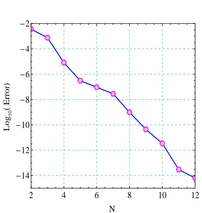
We solve the problem and report the obtained results in Table 1 and Fig-ure 1. In FigFig-ure 1, we plot the L2-norm of the error function in terms of
the various values of the degree of approximation N. Figure 1 shows that the proposed algorithm obtains a good accuracy with suitable values of N. Moreover to make a comparison, we also solve this problem by implementing the well-known Chebyshev collocation method [9, 27] and give the obtained results in Table 1. Based on Table 1, we confirm that the M¨untz-logarithmic polynomials makes faster rate of convergence for the discrete collocation so-lution of this problem compared with the classical Chebyshev polynomials.
Example 3. Consider the following problem:
y(x) =g(x) +x
x
∫
0
ln (x−t)t2y(t)dt,
with
g(x) =x52 −2x 13
2(−13016 + 6930 ln 2 + 3465 lnx)
Galley
Pro
of
Table 1: The numerical errors of Example 2Numerical Errors
N Our Method Chebyshev collocation Method [9, 27]
2 3.61×10⁻³ 1.3×10⁻¹
4 8.13×10⁻⁶ 4.22×10⁻²
6 9.38×10⁻⁸ 2.14×10⁻²
8 9.84×10⁻¹⁰ 1.3×10⁻²
10 3.44×10⁻¹² 8.73×10⁻³
12 6.37×10⁻¹⁵ 6.28×10⁻³
2 4 6 8 10 12
-14
-12
-10
-8
-6
-4
-2
N
Log
10
H
Error
L
Figure 1: ObtainedL2−norm of the error function versusN for Example 2
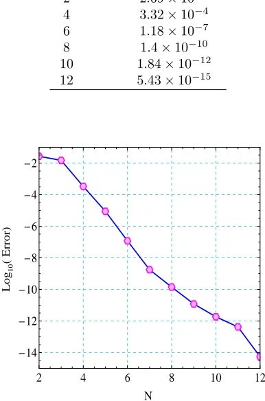
andy(x) =x2√xas the exact solution.
We have calculated the approximate solution with different values ofN
and displayed the obtained results in Table 2 and Figure 2. Table 2 and Figure 2, present theL2-norm of the error functions versusN. As it can be observed although the exact solution has singularity at zero, the numerical errors are decreased with an appropriate rate as the approximation degreeN
is increased.
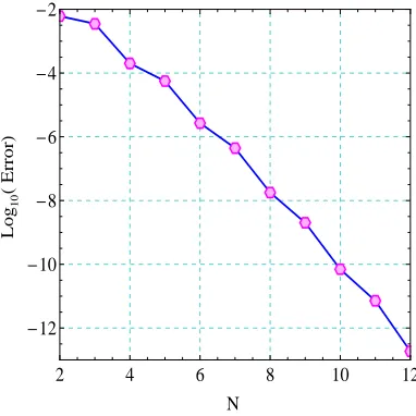
Example 4. Consider the following problem:
y(x) =g(x) +
x
∫
0
Galley
Pro
of
Table 2: The numerical errors of Example 3N Numerical Errors
2 2.69×10⁻² 4 3.32×10⁻⁴ 6 1.18×10⁻⁷ 8 1.4×10⁻¹⁰ 10 1.84×10⁻¹²
12 5.43×10⁻¹⁵
2 4 6 8 10 12
-14
-12
-10
-8
-6
-4
-2
N
Log
10
H
Error
L
Figure 2: ObtainedL2−norm of the error function versusN for Example 3
with
g(x) =ex(1 +γ+ Γ(0, x))+ lnx,
where γ is Euler’s constant with the numerical value≃0.577216 and Γ(0, x) is incomplete gamma function satisfies
Γ(a, z) = ∞ ∫
z
ta−1e−tdt.
Here the exact solution is given byy(x) =ex.
Galley
Pro
of
Table 3: The numerical errors of Example 4N Numerical Errors
2 6.08×10⁻³ 4 2.01×10⁻⁴ 6 2.68×10⁻⁶ 8 1.78×10⁻⁸ 10 6.99×10⁻¹¹
12 1.85×10⁻¹³
results confirm that our scheme provides reliable results for smooth solutions of (1).
2 4 6 8 10 12
-12
-10
-8
-6
-4
-2
N
Log
10
H
Error
L
Galley
Pro
of
6 Conclusion
In this article, we developed a new discrete collocation method based on the M¨untz-logarithmic polynomials as basis functions. Moreover, we used highly accurate Jacobi–Gauss and generalized Jacobi–Gauss quadratures to approximate the integrals with Jacobi and logarithmic weights, respectively. Convergence analysis of the proposed method were presented and some nu-merical examples were illustrated to confirm the applicability of the presented discrete collocation scheme.
References
1. Atkinson, K. E.The Numerical Solution of Integral Equations of the Second
Kind, Cambridge, 1997.
2. Andreasen, M. G. and Mei, K. K. Comments on ”Scattering by conduct-ing rectangular cylinders”, IEEE Trans, Antennas and Propagation, 11 (1963), 52–56.
3. Andronov, I. V.Integro-differential equations of the convolution on a finite interval with kernel having a logarithmic singularity, J. Math. Sci. 79 (1996), no. 4, 1161–1165.
4. Assari, P., Adibi, H., and Dehghan, M. A meshless discrete Galerkin(MDG) method for the numerical solution of integral equations with logarithmic kernels, J. Comput. Appl. Math,267 (2014), 160–181.
5. Banaugh, P. P. and Goldsmith, W. Diffraction of steady acoustic waves by surfaces of arbitrary shape, J. Acoust. Soc. Am.,35 (1963), 1590–1601.
6. Banaugh, P. P. and Goldsmith, W. Diffraction of steady elastic waves by surfaces of arbitrary shape, J. Appl. Mech,30 (1963), 589–597.
7. Ball, J. S. and Beebe, N. H. F. Efficient Gauss-related quadrature for two classes of logarithmic weight functions, ACM Transactions on Mathemat-ical Software,33 (2007), no. 3, Article No. 19.
8. Brunner, H. Collocation Methods for Volterra and Related Functional
Equations, Cambridge University Press: Cambridge, 2004.
9. Canuto, C., Hussaini, M. Y.,Quarteroni, A., and Zang, T. A. Spectral Methods, Fundamentals in Single Domains,Berlin: Springer-Verlag, 2006.
Galley
Pro
of
11. Dom´inquez, V. High-order collocation and quadrature methods for some logarithmic kernel integral equations on open arcs, J. Comput. Appl. Math.,161 (2003), 145–159.12. Guseinov, E. A. and I´linskii, A. S.Integral equations of the first kind with a logarithmic singularity in the kernel and their application in problems of diffraction by thin screens, U. S. S. R. Comput. Maths. Math. Phys., 27 (1987), no. 4, 58–63.
13. Gusenkova,A. A. and Pleshchinskii, N. B. Integral equations with loga-rithmic singularities in the kernels of boundary-value problems of plane elasticity theory for regions with a defect, J. Appl. Maths. Mechs., 64 (2000), no. 3, 433–441.
14. Khader, A. H., Shamardan, A. B., Callebaut, D. K. and Sakran, M. R. A. Solving integral equations with logarithmic kernels by Chebyshev polynomials, Numer. Algorithms,47 (2008), 81–93.
15. Mei, K. K. and Van Bladel, J. G. Low-frequency scattering by rectangular cylinders, IEEE Trans, Antennas and Propagation,11 (1963), 52–56.
16. Mei, K. K. and Van Bladel, J. G. Scattering by perfectly-conducting rectangular cylinders ,IEEE Trans, Antennas and Propagation,11 (1963), 185–192.
17. Mennouni, A.Airfoil polynomials for solving integro-diferential equations with logarithmic kernel, Appl. Math. Comput.,218 (2012), 11947–11951.
18. Milovanovi´c, G. V. M¨untz orthogonal polynomials and their numerical evaluation, Internat. Ser. Numer. Math., 131 (1999), Birkh¨auser Verlag 13asel/ Switzerland.
19. Mokhtary, P.Reconstruction of exponentially rate of convergence to Leg-endre collocation solution of a class of fractional integro-differential equa-tions, J. Comput. Appl. Math., 279 (2015), 145–158.
20. Mokhtary, P.Numerical treatment of a well-posed Chebyshev Tau method for Bagley-Torvik equation with high-order of accuracy, Numer. Algo-rithms, 72 (2016), 875–891.
21. Mokhtary, P. Discrete Galerkin method for fractional integro-differential equations, Acta. Math. Sci., 36 (2016), no. B(2), 560–578.
22. Mokhtary, P. Numerical analysis of an operational Jacobi Tau method forfractional weakly singular integro-differential equations, Appl. Numer. Math., 121 (2017), 52–67.
Galley
Pro
of
24. Muschelischwili, N. I.Singul¨are Integralgleichungen, Akademie-Verlag,Berlin, 1965.
25. Noble, B. Integral equation perturbation methods in low frequency diffraction in R. E. Langer electromagnetic waves, The University of Wis-consin Press, Madison(1963), 323–360.
26. Rivlin, T. J.An Introduction to the Approximation of Functions, United States, 1969.
27. Shen, J., Tang, T., and Wang ,L.-L., Spectral Methods, Algorithms, Analysis and Applications, Springer, 2011.
28. Symm, G. T. An integral equation method in conformed mapping, Nu-mer. Math.,9 (1966), 250–258.
29. Tang, T., McKee, S., and Diogo, T. Product integration methods for an integral equation with logarithmic singular kernel, Appl. Numer. Math., 9 (1992), 259–266.
ﯽﻤﺘﯾرﺎﮕﻟ یﺎﻫ ﻪﺘﺴﻫ ﺎﺑ ﻦﯿﮑﺗ ﻒﯿﻌﺿ رﻮﻄﺑ اﺮﺘﻟو ﯽﻟاﺮﮕﺘﻧا تﻻدﺎﻌﻣ یاﺮﺑ ﻪﺘﺴﺴﮔ ﯽﻠﺤﻣ ﻢﻫ شور
یرﺎﺘﺨﻣ مﺎﯿﭘ
ﯽﺿﺎﯾر هوﺮﮔ ،ﻪﯾﺎﭘ مﻮﻠﻋ هﺪﮑﺸﻧاد ،ﺰﯾﺮﺒﺗ ﺪﻨﻬﺳ ﯽﺘﻌﻨﺻ هﺎﮕﺸﻧاد
١٣٩٧ دادﺮﺧ ٢٣ ﻪﻟﺎﻘﻣ شﺮﯾﺬﭘ ،١٣٩٧ ﺖﺸﻬﺒﯾدرا ٢۶ هﺪﺷ حﻼﺻا ﻪﻟﺎﻘﻣ ﺖﻓﺎﯾرد ،١٣٩۵ رذآ ١۵ ﻪﻟﺎﻘﻣ ﺖﻓﺎﯾرد
ﻦﯿﮑﺗ ﻒﯿﻌﺿ رﻮﻄﺑ اﺮﺘﻟو ﯽﻟاﺮﮕﺘﻧا تﻻدﺎﻌﻣ ﻞﺣ رﻮﻈﻨﻣ ﻪﺑ ﺐﺳﺎﻨﻣ ﻪﺘﺴﺴﮔ ﯽﻠﺤﻣ ﻢﻫ شور ﮏﯾ : هﺪﯿﮑﭼ
رد ﻪﮐ ﺖﺳا ﻦﯾا تﻻدﺎﻌﻣ ﻦﯾا یﺎﻫ ﯽﮔﮋﯾو زا ﯽﮑﯾ .ﺖﺳا ﻪﺘﻓﺮﮔ راﺮﻗ ﯽﺳرﺮﺑ درﻮﻣ ﯽﻤﺘﯾرﺎﮕﻟ یﺎﻫ ﻪﺘﺴﻫ ﺎﺑ رد .ﺖﺳا ﻪﺘﺳﻮﯿﭘﺎﻧ اﺪﺒﻣ رد ﻪﮐ ﺪﻨﮐ ﯽﻣ رﺎﺘﻓر ﯽﻤﺘﯾرﺎﮕﻟ ﻊﺑﺎﺗ ﮏﯾ ﺪﻨﻧﺎﻣ باﻮﺟ لوا ﻪﺒﺗﺮﻣ ﻖﺘﺸﻣ ﯽﻠﮐ ﺖﻟﺎﺣ ﯽﻓﺮﻌﻣ ار ﺪﯾﺪﺟ ﯽﻠﺤﻣ ﻢﻫ دﺮﮑﯾور ﮏﯾ ﯽﻌﻗاو باﻮﺟ ﺎﺑ ﺎﺘﺳار ﻢﻫ ﯽﺒﯾﺮﻘﺗ باﻮﺟ ﮏﯾ ﺖﺧﺎﺳ یاﺮﺑ ﻪﻟﺎﻘﻣ ﻦﯾا نﻮﭼ ،هوﻼﻌﺑ .دﻮﺷ ﯽﻣ هدﺮﺑ رﺎﮑﺑ یا ﻪﯾﺎﭘ ﻊﺑاﻮﺗ ناﻮﻨﻋ ﻪﺑ ﯽﻤﺘﯾرﺎﮕﻟ-ﺰﺘﻧﻮﻣ یﺎﻬﯾا ﻪﻠﻤﺟ ﺪﻨﭼ نآ رد ﻪﮐ ﻢﯿﻨﮐ ﯽﻣ شور ﻪﺑ ﺎﻬﻧآ ﻞﺣ ﺐﻠﻏا ﻪﮐ دﻮﺷ ﯽﻣ ﯽﻤﺘﯾرﺎﮕﻟ یﺎﻫ ﯽﻨﯿﮑﺗ ﺎﺑ ﯽﯾﺎﻫ لاﺮﮕﺘﻧا ﻪﺑ ﺮﺠﻨﻣ دﺮﮑﯾور ﻦﯾا یزﺎﺳ هدﺎﯿﭘ نآرد ﻪﮐ ﻢﯾﺮﺑ ﯽﻣ رﺎﮑﺑ ار ﯽﻤﺘﯾرﺎﮕﻟ نزو ﻊﺑاﻮﺗ ﺎﺑ ﺐﺳﺎﻨﻣ یدﺪﻋ یﺮﯿﮔ لاﺮﮕﺘﻧا شور ﮏﯾ ،ﺖﺳا ﻞﮑﺸﻣ یدﺪﻋ یﺎﻬﺷور رﻮﻈﻨﻣ ﻦﯾﺪﺑ .دﻮﺷ ﯽﻣ ﻪﺒﺳﺎﺤﻣ ﻖﯿﻗد رﻮﻄﺑ ﯽﻤﺘﯾرﺎﮕﻟ نزو ﻊﺑاﻮﺗ ﺎﺑ ﺎﻫ یا ﻪﻠﻤﺟ ﺪﻨﭼ یﺎﻫ لاﺮﮕﺘﻧا ﯽﻣ ﻢﯿﻤﻌﺗ ﯽﻤﺘﯾرﺎﮕﻟ نزو ﻊﺑاﻮﺗ ﺎﺑ یﺎﻬﻟاﺮﮕﺘﻧا یاﺮﺑ اﺮﻧآ ﺲﭙﺳ و هدﻮﻤﻧ یروآدﺎﯾ ار ﯽﺑﻮﮐاژ-سوﺎﮔ یﺮﯿﮕﻟاﺮﮕﺘﻧا ﺐﺳﺎﻨﻣ و ﺖﻗد ﺪﯿﯾﺎﺗ رﻮﻈﻨﻣ ﻪﺑ یدﺪﻋ ﺞﯾﺎﺘﻧ ﯽﺧﺮﺑ و دﻮﺷ ﯽﻣ ﻪﺋارا یدﺎﻬﻨﺸﯿﭘ شور ﯽﯾاﺮﮕﻤﻫ ﺰﯿﻟﺎﻧآ .ﻢﯿﻫد .دﻮﺷ ﯽﻣ ﻪﺋارا یدﺎﻬﻨﺸﯿﭘ شور ندﻮﺑ
؛یدﺪﻋ یﺮﯿﮕﻟاﺮﮕﺘﻧا شور ؛ﯽﻤﺘﯾرﺎﮕﻟ-ﺰﺘﻧﻮﻣ یﺎﻫ یا ﻪﻠﻤﺟ ﺪﻨﭼ ؛ﻪﺘﺴﺴﮔ ﯽﻠﺤﻣ ﻢﻫ شور : یﺪﯿﻠﮐ تﺎﻤﻠﮐ