٭Corresponding Author, Email: [email protected]
An Efficient Method to Control the Amplitude of The
Limit Cycle in Satellite Attitude Control System
M. Sabet Rasekh1, S. K. Y. Nikravesh2* and N. Ghahramani3
1- PhD Educated, Electrical and Electronic Engineering Faculty, Amirkabir University of Technology, Tehran, Iran 2- Professor, Electrical and Electronic Engineering Faculty, Amirkabir University of Technology, Tehran, Iran
3-Associate Professor, Control Group Malek-Ashtar University of Technology, Tehran, Iran
Received 26 July 2015, Accepted 3 January, 2016
ABSTRACT
In this paper, an efficient method is presented to control the attitude of a satellite with ON-OFF actuator. The main objective of this method is to control the amplitude of the limit cycle which commonly appears in the steady state of such systems, while simultaneously by consideration of real actuator constraints, it reduces the fuel consumption of system. The proposed method is a combination of a command modifier (which is based on the set point and the required accuracy of pointing, by means of optimization, it calculates the desired limit cycle), a phase plane controller (PPC) and a compensator (to compensate for the real constraints of the actuator). The effectiveness and outperformance of the proposed method is approved in comparison with the previous methods of attitude control problem through the closed loop simulation and the stability and robustness of the closed loop system is fully analyzed and illustrated by simulations.
KEYWORDS
1. INTRODUCTION
Limit cycle is one of the common characteristics of nonlinear dynamical systems which generally arises in the systems with: uncertain transport delay, ON-OFF actuators, and friction [1-3]. The use of ON-OFF actuators is very common in a large amount of systems such as satellite attitude control systems. In situations in which the amplitude of external noise and disturbance are large, or high control effort is needed, ON-OFF actuators are commonly used. Many of ON-OFF actuators used in attitude control systems are of reaction thruster types. In these actuators, exiting of the gas particles from nuzzles causes a reaction force on system [4].
Attitude control systems, which have ON-OFF actuators, generally converge to a stable limit cycle in their steady state. In the literature, two main reasons are presented for causing this limit cycle. The first reason relates to physical characteristics of ON-OFF actuators. These actuators often have a minimum on-time which means that after the actuator turns ON, there will be no possibility to turn it off in time (thruster valves must stay open over a finite time interval). Therefore, the energy delivered to the system – unlike to the case of using proportional actuators- has a minimum positive value. This cancels the possibility of reaching to the equilibrium state and staying there [2, 5]. The second reason, which causes the limit cycle, is due to the command system. Generally, commanding to the ON-OFF actuator, needs some intermediate systems (such as modulator or bang-bang switches) to change the continuous control command generated by the controller to the ON-OFF command. These intermediate systems generally have a minimum duty cycle or minimum on-time, like the minimum on-time of the actuator, causes a limit cycle. [6]
Obviously, in any satellite attitude control system, a limit cycle is not desirable, because the limit cycle amplitude has an immediate effect on the satellite pointing error1.It means that by increasing the amplitude of the limit cycle, the pointing error will increase. Furthermore, the ON-OFF actuators need propellants; hence, in a limit cycle condition, satellite fuel wastes increases rapidly. Thus, for a certain application, more fuel is needed. The limit cycle frequency and number of pulses in each cycle directly affects loss of fuel. In other words, with increasing frequency of the limit cycle, fuel consumption
1
Pointing error in each control channel is defined as − , where is the command angle and is the angular position of satellite in that channel.
will increase. The Limit cycle also appears in other attitude control systems such as missiles [7].
To reach a stable equilibrium state, the limit cycle, if possible, should be suppressed. In some researches, some proportional actuators (such as momentum exchange devise as reaction wheels), in addition to thrusters, are used in order to suppress the limit cycle [8]. Obviously, additional proportional actuator makes it possible to eliminate the limit cycle; nevertheless, simultaneously, it requires to add drivers, power supply system and controller to the system; this, in turn, leads to an increase in the system weight by occupying a considerable part of the satellite volume, which is not allowed in some applications.
Without proportional actuators, suppressing limit cycle is impossible. Therefore, to avoid the negative role of the limit cycle, its amplitude as well as its frequency should be reduced [2, 9-10]. Of course, it is hard to decrease simultaneously the limit cycle amplitude and its frequency, because they are usually in conflict, i.e. if the limit cycle amplitude reduces, its frequency will increase and vice versa. Hence, a tradeoff is needed between these two criteria [11].
There are two major methods to analyze and control the limit cycle of ON-OFF systems:
1) The describing function method, which is an approximate method based on semi-linearization. In this method, the nonlinear section (i.e. ON-OFF subsystem) is approximated by ratio of Furrier transformation of its output to its sinusoidal input with variable frequency [12-13].
2) Phase plane method, in which, by analyzing the limit cycle in phase plane, proper command for attitude control system is generated [14-16].
The attitude control systems have different types of Limit cycles. The more desirable one is the 2-pulse limit cycle (a limit cycle that has a positive pulse, a negative pulse and two coast regions in each cycle). The 2-pulse limit cycle has the best condition from fuel consumption and robustness point of views [17-18].
and its robustness against satellite and actuator model variations.
The rest of the paper is organized as follows. Section 2 fully presents the statement of the problem. In section 3, the system model components are derived. In section 4 the controller design procedure is fully described, followed by section 5, which presents the effectiveness of the proposed method through simulation. Finally, section 6 concludes the paper.
2. PROBLEM STATEMENT AND ASSUMPTIONS
A satellite attitude control system with ON-OFF actuator, as mentioned before, in steady state converges to a limit cycle and a 2-pulse limit cycle is the most robust type and has the best fuel consumption condition in contrast or with other types of limit cycles. Amplitude of this limit cycle should satisfy pointing requirement of the system. On the other hand, the limit cycle frequency in order to have less fuel consumption, should decrease as big as possible.
Other assumptions of this problem are as follows. The satellite is rigid and non-spinning. The thrust force delivered by actuators are the only moment signal acting on the body. The sensors have sufficient resolution and their noises are negligible. The actual ON-OFF actuators have some imperfections such as delay, minimum on-time and having dynamics in both turning ON and OFF phases. Therefore, design of the proper controller should be done considering these constraints.
In order to design an attitude control system, we are required to have in advance both the angular position and angular velocity of the system in all three control channels. In this paper, it is assumed that these relevant variables are measured through a precise inertial navigation system which will be in turn to the control system.
The main objective here is to design this controller to fulfill 1) an on-orbit stabilization with a fine attitude regulation in which the pointing error should not exceed a predefined value; 2) the closed loop system should converge to a 2-pulse limit cycle with a minimum fuel consumption subject to the aforementioned assumptions. In the next section, the mathematical model of the attitude control system and ON-OFF actuators are represented.
3. MODELING
A. Satellite Attitude Control System Model A satellite attitude control system model is composed of the following six coupled first order nonlinear differential equations [8]:
̇= − +
̇= − +
̇= − +
̇ = + tan ( sin + cos )
̇ = cos − sin
̇ = ( sin + cos )
(1)
In which [ ] and [ ] are Euler angels and system angular velocities in roll, pitch and yaw channels,
respectively. [ ] , [ ] and,
[ ] are system inertial momentums, actuators output thrust levels and control commands in each channel, respectively. Obviously, if approaches90°, a singularity will happen in the system. In such conditions, the above model known as Euler angle model is not suitable to use and the quaternion based model is more convenient [8]. Since the Euler angles used in this paper are far from the singularity point, the Euler angles model is used to design the controllers and in addition, the linearized model of the system can be used in this case. In the linearized case, the attitude control equation in each channel is described as: [19]
̈ = (0) = ̇(0) = (2)
where and are the angular position and angular velocity at the actuator switching moment, is the actuator output thrust level, and is a constant coefficient depends on the inertial momentum.
B. The ON-OFF Actuator Model
In the baseline problem considered in this paper, the actuator switchings are subject to some restrictions as stated below. The real cold-gas actuator has a delay time , a rise time, , a minimum on-time, , and a fall time, in each pulse. The actuator behavior in rise time and fall time can be approximated by a first order or second order polynomial function, based on the accuracy required. During the delay time and the minimum-on-time the actuator's output is considered constant. From now on, the sum of these times is named as minimum pulse width,
∗.
To obtain ∗ in real cases we should run some experimental tests for determining the proper values of rise time, delay time, fall time and minimum-on-time in an average sense.
4. THE ATTITUDE CONTROLLER DESIGN
According to the modeling of the plant and the actuator in the previous section, the controller design procedure is presented in this section. First, the cost function, which is the base of the controller optimality, will be described, and then, by solving the optimal control problem, a suboptimal limit cycle is derived. Then the controller is presented and finally a compensator to compensate the actuator constraints is represented.
A. Defining the Cost Function
In the method presented in this paper, for the system to have a limit cycle with desired characteristics, first the modification of command is done. It means that rather than an equilibrium state, the limit cycle trajectory with desired characteristics will exert to the system as a modified command. Then, a controller will be designed to force the system to track this optimal limit cycle. Indeed, the regulation problem will convert to a tracking problem. Albeit this change makes the problem more difficult, it makes it possible to reach the control goals. Furthermore, it is obvious that the robustness of the method against noise and model changes will improve.
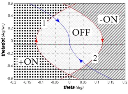
As mentioned earlier a 2-pulse limit cycle has a positive pulse (L1), a negative pulse (L3) and two OFF regions or coast region (L2, L4), as shown in Fig. 1. As this figure depicts, in the coast region, the angular velocity of the system is constant and in the conditions that the actuator is on, the trajectory of the system is indeed a parabolic path.
To have an optimal 2-pulse limit cycle, a cost function is defined as:
= + (4)
= (5)
= ( + ) (6)
in which and are the fuel consumption in regions L1 and L3 and and are the coast times of L2 and L4 segments, respectively. To optimize this cost function, one can divide it into two separate sections. Thus, optimization can be done through two separate optimization problems in ON and OFF regions as stated below.
min & ( ) & min & ( ) (7)
The optimization should be done according to both the required pointing accuracy and the plant constraints.
B. The Suboptimal Limit Cycle
To have a 2-pulse limit cycle as shown in Fig. 1, inequalities (8) and (9) should hold.
̇ ̇ ≤0 (8)
̇ − ̇ ≥ (9)
where ̇ and ̇ are the angular velocity in L4 and L2 respectively. Inequality (8) is obtained according to the characteristics of the 2-pulse limit cycle which has a positive and a negative pulse. Therefore, the angular velocity in one of the coast regions is positive and in the other one is negative. Inequality (9) is obtained based on the actuator minimum ON-time. As mentioned earlier, the minimum ON-time of the actuator makes changes in angular velocity of the plant in each pulse get greater than
a minimum value equals to with =∫∗ . In
addition to these constraints, the maximum value of the attitude error is one of the other constraints that should be considered. Obviously, if the system converges to a limit cycle with zero mean and an amplitude equals to the maximum permissible attitude error, the attitude error constraint should be met. Thus, if a controller is able to satisfy these three constraints simultaneously, it is guaranteed that the system converges to a desirable two-pulse-limit cycle. Now, with regard to these constraints, the optimization problem is solved as stated below. According to equation (2), the system’s trajectory in positive, negative and OFF regions can be described respectively as:
= ̇ + (10)
=− ̇ + (11)
= ̇ + (12)
Thus, if the limit cycle's amplitude becomes equal to A, the trajectories L1 and L3 can be described as (13) and (14), respectively.
L1: = ̇ − (13)
L3: =− ̇ + (14)
Hence, and are obtained as:
=− ̇ + 2 ̇ (15)
=− ̇ + 2 ̇ (16)
and becomes
=( ̇ ̇̇ ̇)(̇ ̇ ) (17)
Now, by differentiating equation (17) (for briefness, the straightforward procedure of differentiating and the mathematical operations are omitted), the optimal value of this function will be obtained when either θ̇ orθ̇ is zero; this means that if the angular velocity of the system becomes zero and the actuator is OFF, theoretically, the system should keep its state fixed. It is obvious that this situation will not be possible in real world. Therefore, this problem has no optimal solution though it is possible to obtain a suboptimal solution.
On the other hand, in order to minimize , the width of each pulse ( and ) no matter positive or negative must be made equal to the minimum pulse width and
under the constraint mentioned in (9) ( ̇ − ̇ = ).
Therefore, the desired limit cycle can be explained as
1) Trajectory described by = ̇ − ; (positive
pulse)
2) Trajectory described by ̇= ̇ ; (coast region)
3) Trajectory described by = − ̇ + ;
(negative pulse)
4) Trajectory described by ̇ = ̇ ; (coast region)
in which ̇ or ̇ should be as close as possible to axis and also the condition (9) should be satisfied. The valueA is the desired limit cycle amplitude which is equal to the maximum allowable pointing error. Now, by having the desired trajectory in hand, a controller is needed to bring the system trajectory to this desired limit cycle.
C. The Controller Design
The goal here is to design a controller which leads the system to the desired limit cycle. A good choice for this purpose would be a phase plane controller (PPC). A PPC generates the ON-OFF command based on the comparison between the state variables of the system (the angular position and the angular velocity) and some switching curves. The PPC controller has some advantages such as:
· This controller directly generates the desired ON-OFF commands. Thus, there is no need to an intermediate subsystem (such as modulator) to change the control command to an ON-OFF command.
· The PPC controller can be simply implemented on flight computers.
· Since the suboptimal limit cycle was obtained based on the phase plane trajectories, the PPC design is much simpler than the other control methods.
· The PPC is able to provide a good feeling of dynamics and physical performance of the system for the user.
To design the PPC controller, the following steps should be taken:
· Two switching curves according to eq. (13) and (14) are taken since the optimized limit cycle is determined with these equations.
· The controller should somehow operate that the system from any initial condition go toward the switching curves. Therefore:
§ If the initial state of the system is between the two switching curves, considering that the error of the attitude of the system is less than the allowable limit, the actuator remains off till the state reaches one of the switching curves. § If the initial condition is out of the area
between the switching curves, since the error is exceeded from the allowable error limit, the state should bring to one of the switching curves, using bang-off-bang command.
· Having reached the switching curves, in a suitable timing, the required commands must be given to have the desired limit cycle. For this reason, two
off-boundaries are considered in ̇ = ± and another
curves and the actuator is OFF, an ON command (L1) or –ON command (L2) should be executed.
To have a desired limit cycle, the PPC controller should consist of two switching curves described by (13) and (14) and two OFF boundaries given by ̇ = ± .
When the system trajectory meets this off boundary, the actuator should turn off. For more explanations, this controller is depicted graphically in Fig. 2. This controller works well using an ideal actuator, and in the presence of uncertainties or real constraints in actuators, a compensator might be used along with the PPC controller in order to improve its performance.
Fig. 2.Switching curves of optimal controller ( : = ̇ − : = − ̇ + )
D. Design of a Compensator Based Constrained Controller
As mentioned before, the On-OFF actuators have some imperfections and constraints due to their physical nature [20-21]. Since in the steady state the actuator generates pulses with a minimum pulse width, the actuator constraints have more effects on the system. Thus, it is necessary to consider these constraints to design a proper controller. In this section, a method will be introduced for compensating the effects of the actuator real constraints. The stages of compensation for dynamics of the actuator in the ON mode are presented here, and the other compensations are omitted for the briefness.
1) Delay time: during the delay time, the satellite moves on the trajectory (12). Therefore, if the actuator has a seconds delay, a compensation term equal to ̇ should be added to the switching curve.
2) Rise time: after elapsing the delay time, the actuator output starts to increase and after a small period of time, , it reaches to its nominal value. If the thruster output in the rise time is
approximated by a linear function, then (18) and (19) would hold.
̈ = (18)
= + ̇ + (19)
At the time instance = 0, we will have the initial values = , ̇ = ̇ and ̈= 0, and at the time = we have:
̇( ) = + ̇ (20)
( ) = + ̇ + (21)
For ( ) to be on the trajectory (13), the following equation should be satisfied:
( ) = + ̇ + = + ̇ − (22)
Therefore, when the actuator’s output level reaches its nominal value, the states will lie on (13) whenever satisfies (23).
= ̇ − − ̇ − (23)
The comparison between (13) and (23) shows the
necessity of moving the switching curve by + ̇ .
For the other constraints the same procedure should be followed.
3) The fall time: In the fall time, the actuator output will decrease for seconds in order to reach zero.
To compensate for this, a term should be
added to the switching curve.
4) The minimum impulse of the actuator: as mentioned before, when the actuator turns ON, it is impossible to turn it off immediately, so the pulses delivered by the actuator have a minimum width. In this case, the energy delivered by the actuator in a pulse with minimum width is defined as the actuator minimum impulse as:
≜ ∫ (24)
in which is the thrust level of the actuator output. Because of this minimum impulse, the minimum value of variations in the angular velocity is equal to ⁄ . On the other hand, the actuator impulse during turning off is defined by:
=∫ μdt (25)
in the opposite directions, two nuzzles stand in the opposite directions. One of them makes a positive pulse, while the other one makes a negative pulse. In this matter, in order to prevent rapid loss of energy, the thrusters are designed in a way to obstruct the output valves of the thrusters from opening at the same time. In addition, for the actuators, direct switching from ON state (positive pulse) to -ON state (negative pulse) and vice versa is not possible and first the actuator should turn off and then it switches to the opposite pulse. Thus, often a coast region between two opposite ON regions is needed. In addition to satisfying this constraint, this region eliminates the system chattering. The width of this coast region is determined so that when an ON command reaches just before a switching curve, the actuator will be able to turn off before reaching the reverse ON region.
In each actuator, some of such physical constraints exist or they can be neglected based on some certain conditions. Thus, summary of compensations are represented in Table 1.The first set of the equations in Table 1 is related to the switching curve in the boundary of coast region and the ON region, while the second set is related to the boundary of coast and -ON regions.
TABLE 1.THE EFFECT OF ON-OFF ACTUATOR COMPENSATION ON THE SWITCHING CURVES IN THE PPC
CONTROLLER
1st set 2ndset
Ideal switching
curve =2 ̇ − =−2 ̇ +
delay =
2 ̇ − − ̇ =−2 ̇ + − ̇
Rise time =
2 ̇ −24 − 1 2 ̇
−
=−2 ̇ +24 −12 ̇
+
Fall time
̇= −
2 ̇=− +2
̇=
2 ̇=−2
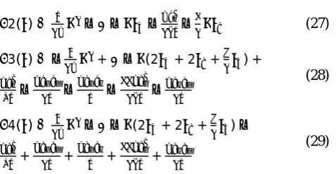
The phase plane controller switching curves with compensator are given below.
1( )≜ − ̇ + − ̇ + − ̇ (26)
2( )≜ ̇ − − ̇ − − ̇ (27)
3( )≜ − ̇ + − ̇(2 + 2 + ) +
− − − − (28)
4( )≜ ̇ − − ̇(2 + 2 + )−
+ + + + (29)
As mentioned earlier, a coast region is needed between two regions with opposite pulses; hence, the number of switching curves are indeed reduced to four.
E. Summary of the Control Algorithm
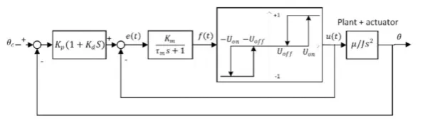
This paper presents a three step method to control the satellite attitude with a predetermined accuracy and minimum fuel consumption. In the first step, based on the control command and desired accuracy, an optimization problem is solved according to the constraints of the plant dynamics, and the desired limit cycle is calculated (the command modifying stage). In the second step, a PPC controller is designed in a way that it can bring the system to the desired limit cycle. Finally, in the third step, this ideal controller is combined with a compensator to compensate for the physical constraints of the actuator and to exert the control command. The phase plane controller with compensator is shown in Fig. 3, whilethe block diagram of this controller is presented in Fig.4.
Fig. 3. PPC controller with compensator
The proposed method can be summarized as:Ina satellite attitude control system using non-ideal ON/OFF actuators -with output thrust level, µ, delay time , rise time, , minimum on-time, , fall time, , and moment
of inertia of the desired control channel, J, a phase plane controller with switching curves described by equations (26)-(29) and the off boundaries± / and± is able to
bring the system to a 2-pulse limit cycle with a minimum fuel consumption and an amplitude equals to A (the maximum allowable error of the angular position). In order to implement the proposed controller in a flight computer, one can use the following algorithm.
ALGORITHM 1
1) Determine the desired limit cycle based on the maximum allowable angular position error as well as system equations (the result of the section 4.2)
2) Calculate the switching curves T1-T4 from equations (26)-(29).
3) Calculate the control command (U) from the following rules:
Ifθ> 1&θ ≥T4⇒U =−1
Ifθ< 4&θ> 1 ⇒U =−1
Ifθ< 2&θ ≤T3⇒U = 1
Ifθ< 2&θ> 3&θ̇< 0⇒U = 1
OtherwiseU = 0
4) If the system trajectory crosses the OFF boundary, turn the actuators OFF.
If θ̇(t−2) > / and θ̇(t−1) ≤m/J ⇒U = 0
If ̇( −2) > / & ̇( −1) ≤ / ⇒ = 0
If ̇( −2) ≤ / & ̇( −1) > / ⇒ = 0
5) Apply the command input U to the actuator.
The method presented in this paper has many advantages such as:
1) Satisfying the required pointing accuracy of the system and minimum fuel consumption simultaneously. Because the index of the optimization problem is a function of the fuel consumption, and the maximum error is considered as a constraint, this method is able to
satisfy both the error limit and the minimum fuel consumption.
2) Real-time implementation: since the parametric switching curves equations are computed offline, the computation time of online equations will not be considerably high. In addition, the switching curves equations can be simply implemented in flight computers by employing Algorithm 1. Hence, the real time tuning of the controller can be properly done.
5. SIMULATIONSAND RESULTS
To illustrate the efficiency of the proposed controller, the system is implemented in MatLab Simulink and the simulation results are compared with two common methods for attitude control of a satellite: a PID controller with PWPF modulator and a bang-bang controller with dead zone described in the following. After this, the closed loop system with the proposed controller is simulated in three control channels. Parameters of the plant and the actuator for these simulations are presented in Table 2.
TABLE 2. PARAMETERS USED IN SYSTEM SIMULATION
J µ
(N)
Sampling time (sec)
td (sec)
tr (sec)
to
(sec) tf(sec)
700.8 30 0.01 0.02 0.13 0 0.28
A. PID Controller with PWPF Modulator
This method, which is one of the most widely used satellite attitude control method, consists of a PID controller and a PWPF modulator. The modulator changes the continuous control signal to a pulse train of on/off command. The width and the frequency of these pulses changes based on the input amplitude. Fig. 5 shows the block diagram of the closed loop system. The parameters of this modulator are adjusted based on the method given on [6] to reach a limit cycle with an amplitude equal to 0.5 degree. These parameters are presented in Table 3.
TABLE 3. PARAMETERS OF PID CONTROLLER WITH PWPF
Kd Ki Kp Kpre Km τm Uoff Uon
12 .2 7.008 1.75 4.3 .1 .4 .85
B. PID Controller with a Bang-Bang Switch In this method, a bang-bang switch with dead zone converts the control signal to the proper ON-OFF command to exert to the actuator. The block diagram of this method is depicted in Fig. 6.The coefficients of this controller are adjusted based on the method given in [6] and presented in Table 4.
Fig. 6. PID controller with bang-bang switch
TABLE 4. PARAMETERS OF PID CONTROLLER & BANG-BANG SWITCH
Kd Ki Kp
6.7 2 2.4 0.049
C. Simulation Results
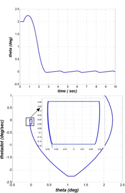
As previously mentioned, one of the major advantages of the proposed method is to satisfy the required pointing accuracy of the system. This advantage was analytically proven above, and in this section it is shown through simulations. For this reason, here the system with the proposed controller is setup in order to have a maximum error of order 0.05 degrees.
As shown in Fig. 7, the system converges to the desired limit cycle with the acceptable error and transient time. In addition, the PPC controller with compensator satisfies the real actuator limitations.
In the Fig. 8, the outputs of the controller and the actuator are presented (the output of the controller is scaled through multiplying by 30 to be comparable with that of the actuator). As expected, at first, the controller produces some pulses conducting the system toward the desired limit cycle in a bang-off-bang mode, and then, by creating pulses with minimum pulse width, it keeps the system in the limit cycle mode. It can be seen that the actuator's output follows the control command with a delay.
In the previous attitude controllers, unlike to the proposed method, converging to a limit cycle with a predetermined amplitude and minimum frequency is not possible. Thus, by trial and errors, the parameters of these controllers are adjusted to have a limit cycle with 0.5 degree amplitude (Fig. 9).
Fig. 7. System response with the proposed controller
Fig. 8. The output of the controller and the actuator
bang-bang and PWPF modular methods. Indeed, periods of limit cycle resulted from these three methods are: 34.5, 9.36 and 9.59 seconds, respectively. This shows that fuel consumption in the proposed method is much lower than the other methods.
Fig. 9. Comparison of 3 control methods: (A) in phase plain (B) in time domain
The fuel consumption in systems with ON/OFF actuators is directly proportional to the duration of time at which the actuator is ON. To compare the fuel consumptions of these systems, they are set to have a limit cycle with similar amplitudes. In doing so, the ON-time of actuators in 100 seconds of the steady state limit cycle are given in Table 5 for the purpose of comparison. As can be easily seen the fuel consumption in the proposed method is significantly less than that of the other methods. It should be mentioned that in the lower range of limit cycle amplitude, the amount of decrease in the fuel consumption in the proposed method is much bigger.
TABLE 5. THE ON-TIME OF 3 CONTROL METHODS IN 100 SECONDS
Case no.
Limit cycle amplitude
Proposed method
PID+
PWPF
PID+ bang-bang switch
1 A=0.5 deg. 3.44 12.25 12.04
2 A=0.3 deg. 8.32 40.75 52.23
3 A=0.7 deg. 2.03 8.35 7.74
4 A=0.9 deg. 1.43 4.21 4.16
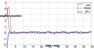
D. Three Channel Simulation
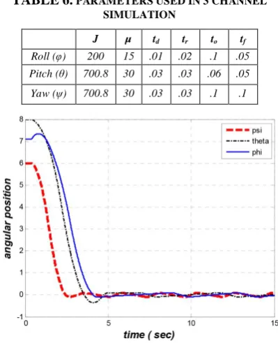
In this section, the satellite attitude control system with the proposed controller is simulated in three control channels. The goal of the system is to have a maximum pointing error less than 0.1 degree. The coefficients and the parameters used in nonlinear three channel simulations are presented in Table 6. As depicted in Fig. 10, using this method, the system can converge through 3 control channels to a limit cycle with the desired accuracy.
TABLE 6. PARAMETERS USED IN 3 CHANNEL SIMULATION
J µ td tr to tf
Roll (φ) 200 15 .01 .02 .1 .05
Pitch (θ) 700.8 30 .03 .03 .06 .05
Yaw (ψ) 700.8 30 .03 .03 .1 .1
Fig. 10. Three control channels' simulation using the proposed controller
In the Fig. 11, the output of the controller is shown. As easily observed, the controller generates pulses with minimum width which makes the duty cycle (the ratio of the on-time of the actuator to the period of the limit cycle) very small, and as a result, the fuel consumption is remarkably reduced.
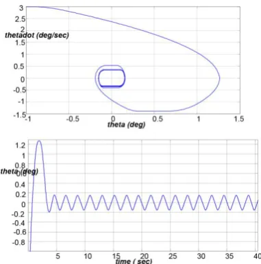
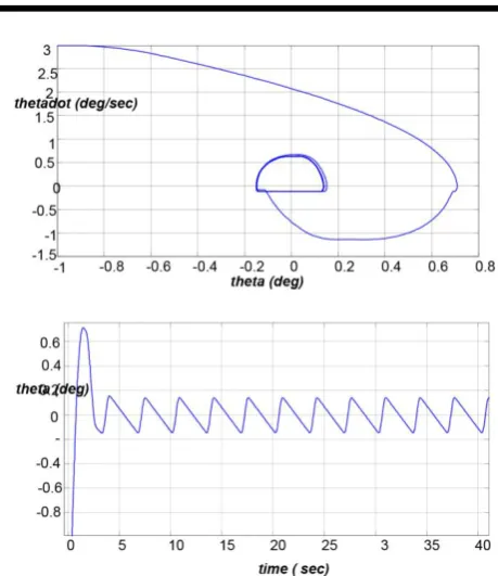
E. Stability Analysis
To analyze the stability of the closed loop system, assume that the system's initial condition is X0( = , ̇= ̇ ).By using the proposed controller, the system trajectory crosses the points X1 to X6, as depicted in Fig. 12, and finally, it converges to the limit cyclespecified with points X3 to X6. From this figure, it can be concluded that for all of these initial conditions, the system has similar results and the system trajectory will move toward the origin and converge to a limit cycle around the origin. If the trajectory is separated from the limit cycle, the controller will take it back to the limit cycle again. For this reason, although the origin of the phase plane is not stable in the sense of Lyaponuve, the closed loop system is BIBO.
Fig. 12. Stability analysis of the closed loop system
F. Robustness Analysis
The uncertainties and disturbances in satellite attitude control systems are of various form. The parameters which would consist of uncertainties are the moment of inertia of the satellite, the actuator output thrust level and the measurement of the angular position and the angular rate could have some noise.
To analyze the robustness of the proposed method, the controller is designed by the nominal values of the parameters and then the uncertainties are inserted in the simulations and the effect of using the nominal controller on the real system is studied. Before seeing the analysis results, with a common sense it is obvious that the system with the proposed controller is very robust in contrast with the model uncertainties and noises because of the first step of the control method (command modifying step) which wants to force the system with any conditions and parameters values to track a predefined limit cycle. This claim is being investigated below.
i. Robustness Analysis in One Channel
First assume that the nominal values of parameters of the system is as in Table 6 and the desired amplitude of
the limit cycle is 0.15 degree. The nominal system's output is illustrated in Fig. 13.
Fig. 13. The response of the nominal system
a) Uncertainty in the Moment of Inertia
Suppose that the actual value of the moment of inertia is 10% less than its nominal value. The output of the system with the proposed controller is presented in Fig. 14. As it can be seen in the steady state there is no mentionable difference between the nominal and perturbed system's response but the perturbed system has a bit more fast transient response with more overshoot because of its less moment of inertia. Now, suppose that the actual value of the moment of inertia is 20% more than its nominal value. As it can be seen in Fig. 15 the system has less overshoot but it has the same limit cycle, yet. It means that the system is robust against the variations in the moment of inertia.
Fig. 15. The effect of a 20% change in moment of inertia
b) Uncertainty in the Output Level of the Actuator Assume that the actual output of the thruster is 10% more than its nominal value. As it is seen in Fig. 16 the steady state limit cycle has the same amplitude as the nominal system. Now, suppose that the actual output thrust level of the actuator is 20% less than its nominal value. The simulation result is depicted in Fig. 17.
Fig. 16. 10% perturbations in the thruster output level
Fig. 17. -20% perturbations in the thruster output level
c) Noise in the Measurements
Assume that there is a white noise with a 0.05 deg/sec amplitude in measurements of the angular rates. The results are presented in Fig. 18. It should be mentioned that 0.05 deg/sec is a very large amount of noise in the real problems. It can be seen that the system mean value of the amplitude of variations is just near 0.15 degree.
Fig. 18. Effect of noise in the angular rate measurement
ii. Robustness Analysis in 3 Channels
Fig. 19. The nominal system response
a) Perturbations in the Moment of Inertia
Assume that the actual value of the moment of inertia in yaw channel is 50% less than its nominal value. As it can be seen in Fig. 20 the proposed controller has a great robustness against the variations in the system parameters. In Fig. 21 it is assumed that the actual value of the moment of inertia in pitch channel is 50% more than its nominal value where in Fig. 22 the moment of inertia in roll channel has a 50% variations.
Fig. 20.Perturbations in yaw channel’s moment of inertia
Fig. 21. Perturbations in pitch channel’s moment of inertia
Fig. 22. Perturbations in roll channel’s moment of inertia
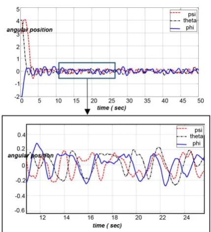
b) Noise in the Measurements
For the investigation of the effect of measurement noise on the system first assume that there is a white noise with a 0.05 deg/sec amplitude in measurements of p which its result is illustrated in Fig. 23. Then assume that there are white noise errors on the measurement of all the p, q and r with amplitude equals to 0.1 deg/sec. The output of the system is depicted in Fig. 24. It can be seen that the system does well in the noise rejection.
Fig. 23. Effect of white noise with a 0.05 deg/sec amplitude in measurements of p
Fig. 24. Effect of white noise error on the measurement of all the p, q and r with amplitude equals to 0.1 deg/sec
c) Uncertainty in the Thruster Output Level
system there is not a limit cycle in the system and a kind of fluctuation will appear in the system which amplitude should be concerned,
Fig. 25. The effect of uncertainty in thruster output level
6. CONCLUSIONS
This paper presented an effective method for attitude control of a satellite with ON-OFF actuator. The main objective of the proposed controller was to bring the system to the steady state limit cycle, which always appears in satellite ACS, with a minimum fuel consumption for an appropriately pre-specified amplitude and minimum number of switchs. The proposed controller consists of the following three parts.
1) A command modifier based on i) the desired pointing accuracy, ii) the input command and iii) the system constraints, calculated the optimal limit cycle and then exerted it to the system.
2) A phase plain controller (PPC) which ideally brings the system to the optimal limit cycle.
3) A compensator compensated for the physical constraints of the actuator.
The capabilities of the proposed controller were analytically proven and validated through simulations in both one and three control channels. Finally, the advantages of the proposed method in comparison with those of the other common attitude control methods were confirmed using simulation and its stability and robustness is studied too.
ACKNOLEDGMENT
We would like to show our gratitude to the Professor M. B. Menhaj (Professor of Electrical and electronic engineering faculty, Amirkabir University of Technology) for sharing his pearls of wisdom with us during the course of this research.
REFERENCES
[1] H. Olsson and K. J. Astron, “Friction Generated Limit Cycles,” IEEE Transaction on Control Systems and Technology, Vol. 9, No. 4, 2001.
[2] Y. J. Huang and Y. J. Wang, “Limit Cycle Analysis of Electro-Hydraulic Control Systems with Friction and Transport Delay,” in World Congress on Intelligent Control and Automation, 2000.
[3] M. Tanelli, et al, “Limit Cycles Analysis in Hybrid Anti-Lock Braking Systems,” in IEEE Conference on Decision and Control, 2007.
[4] S. Adler, A. Warshavsky and A. Peretz, “Low-Cost Cold-Gas Reaction Control System For Slohsat FLEVO Small Satellite,” journal of Spacecraft Rocket, Vol.42, No.2, 2005.
[5] Robert N. Clark, “Limit Cycle Oscillation in Pulse-Modulated Systems,” Journal of Spacecraft, Vol. 6, No. 7, 1969.
[6] T. D. Krovel, “Optimal Tuning of PWPF Modulator for Attitude Control,” M.S. Thesis, Department of Engineering Cybernetics, Norwegian University of Science and Technology, 2005.
[7] Philip C. Calhoun and Eric M. Queen, “Entry Vehicle Control System Design for the Mars Smart Lander,” in AIAA Atmospheric Flight Mechanics Conference, Monterey, California, 2002.
[8] Marcel J. Sidi, “Spacecraft Dynamics and Control,” Cambridge University Press,1997.
[9] B. F. Wu and J. W. Perng, “Limit Cycle Analysis of PID Controller Design,” American Control Conference, 2003.
[10] J. W. Perng, B. F. Wu, H. I. Chin, and T. T. Lee, “Limit Cycle Analysis of Uncertain Fuzzy Vehicle Control Systems,” in IEEE Conference on Networking, Sensing and Control, 2005.
[11] J. Mendel, “On-Off Limit-Cycle Controllers for Reaction-Jet-Controlled Systems,” IEEE Transactions on Automatic Control, Vol. 15, No. 3, 1970.
[12] B. F.Wu, J.W. Perng, and J. I. Chin, “Limit Cycle Analysis of Nonlinear Sampled-Data Systems by Gain-Phase Margin Approach,” J. Franklin Inst., Vol. 342, 2005.
[13] C. C. Cheng and C. H. Huang, “On the Limit Cycle of The Underwater Vehicle Control System,” in Int. Symposium Underwater Technol., 1998.
[14] V. E. Haloulakos, “Thrust and Impulse Requirements for Jet Attitude Control Systems,” J. Spacecraft, 1964.
[15] M. H. Kaplan, “Modern Spacecraft Dynamics and Control,” Wiley press, New York, 1976.
in AIAA Guidance, Navigation and Control Conference, 1992.
[17] R.N. Clark, “Limit Cycle Oscillation in a Satellite Attitude Control System,” Automatica, Vol. 6, 1970.
[18] M. J. Abzug, el al., “A Time Optimal Attitude Control System Designed to Overcome Certain Sensor Imperfection,” Guidance and Control II, edited by R. Langford, Elsevier, 1964.
[19] Sang W. Jeon and Seul Jung, “Hardware-in-the-Loop Simulation for The Reaction Control System Using PWM-Based Limit Cycle Analysis,” IEEE
Transactions on Control Systems Technology, Vol. 20, No. 2, Mar. 2012.
[20] A. R. Mesquita, K. H. Kienitz and E. L. Rempel, “Robust Limit Cycle Control in an Attitude Control System with Switching-Constrained Actuators,” in The 47th IEEE Conference on Decision and Control, Cancun, Mexico, Dec. 9-11, 2008.