Solving a non-linear optimization problem in the presence of Yager-FRE constraints

journal homepage: http://jac.ut.ac.ir

Solving a non-linear optimization problem in the

presence of Yager-FRE constraints

Amin Ghodousian

, Abolfazl Javan

and Asieh Khoshnood

Department of Engineering Science, College of Engineering, University of Tehran.

2,3_{Department of Algorithms and Computation, University of Tehran.}

ABSTRACT ARTICLE INFO

Yager family of t-norms is a parametric family of con-tinuous nilpotent t-norms which is also one of the most frequently applied one. This family of t-norms is strictly increasing in its parameter and covers the whole spec-trum of t-norms when the parameter is changed from zero to infinity. In this paper, we study a nonlinear op-timization problem where the feasible region is formed as a system of fuzzy relational equations (FRE) defined by the Yager t-norm. We firstly investigate the resolution of the feasible region when it is defined with max-Yager composition and present some necessary and sufficient conditions for determining the feasibility and some

Article history:

Received 12, January 2018 Received in revised form 5, May 2018

Accepted 27 May 2018

Available online 01, June 2018

Keyword: Fuzzy relational equations; nonlinear optimiza-tion; genetic algorithm

AMS subject Classification: 05C78.

∗_{Corresponding author: A. Ghodousian. Email: [email protected]} †_{[email protected]}

‡_{[email protected]}

1

Abstract continued:

procedures for simplifying the problem. Since the feasible solutions set of FREs is non-convex and the finding of all minimal solutions is an NP-hard problem, conventional nonlinear programming methods may involve high computation complexity. For these reasons, a method is used, which preserves the feasibility of new generated solutions. The proposed method does not need to initially find the minimal solutions. Also, it does not need to check the feasibility after generating the new solutions. Moreover, we present a technique to generate feasible max-Yager FREs as test problems for evaluating the performance of the current algorithm. The proposed method has been compared with Lu and Fangs algorithm. The obtained results confirm the high performance of the proposed method in solving such nonlinear problems.

2

Introduction

In this paper, we study the following nonlinear problem in which the constraints are formed as fuzzy relational equations defined by Yager t-norm:

min f(x) Aϕx=b x∈[0,1]n

(1)

whereI ={1,2. . . m},J ={1,2. . . n},A = (aij)m×n, 0≤aij ≤1, (∀i∈I and ∀j ∈

J) is a fuzzy matrix, b = (bi)m×1, 0 ≤ bi ≤ 1 (∀j ∈ I) is a m-dimentional fuzzy

vector, and ϕ is the max-Yager composition that is ϕ(x, y) = TP

Y (x, y) = max{1−

[(1−x)p+ (1−y)p]1p _,0} _{in which p >0.}

if ai is the i’th row of matrix A, then problem 1 can be expressed as follows:

min f(x)

ϕ(ai, x) = bi, i∈I

x∈[0,1]n

(2)

where the constraints mean:

ϕ(ai, x) = max

j∈J {ϕ(aij, xj)}= maxj∈J {T P

Y (aij, xj)}

= max

j∈J {max{1−[(1−aij)

p_{+ (1−x} j)p]

1

p,0}}

=bi, ∀i∈I

(3)

As mentioned, the family {T_YP} is strictly increasing in p. It can be easily shown that Yager t-norm TP

infinity and converges to Drastic product t-norm [8] as p approaches zero. Also, it is interesting to note thatT1

Y(x, y) = max{x+y−1,0}, that is, the Yager t-norm is converted

to Lukasiewicz t-norm if p = 1. In [43] three feature types were presented based on the concept of information set for face recognition, which includes sigmoid and energy features, two features, viz. effective information set features-I and features-II and their combinations using t-norms and s-norms of Hamacher and Yager, and two hybrid features called Gabor-information set features and wavelet-information set features. In [46] the authors used Yager t-norm and t-conorm to investigate the performance of Fuzzy inference procedure of Fuzzy ID3 algorithm. In [47], the authors generalized a fixed-point theorem in fuzzy metric spaces by using a class of continuous t-norms known as ω-Yager t-norms, which was successfully used to prove the existence and uniqueness of solution for the recurrence equation associated with the probabilistic divide and conquer algorithms. The problem to determine an unknown fuzzy relation R on universe of discourses U×V such that AϕR =B, where A and B are given fuzzy sets on U and V, respectively, and ϕ is an composite operation of fuzzy relations, is called the problem of fuzzy relational equations (FRE). Since Sanchez [54] proposed the resolution of FRE defined by max-min composition, different fuzzy relational equations were generalized in many theoretical aspects and utilized in many applied problems such as fuzzy control, discrete dynamic systems, prediction of fuzzy systems, fuzzy decision making, fuzzy pattern recognition, fuzzy clustering, image compression and reconstruction, fuzzy information retrieval, and so on [5,11,24,28,40,44,45,48,51,59,61,67]. For example, Klement et al. [31] presented the basic analytical and algebraic properties of triangular norms and important classes of fuzzy operators generalization such as Archimedean, strict and nilpotent t-norms. In [50] the author demonstrates how problems of interpolation and approximation of fuzzy functions are converted with solvability of systems of FRE. The authors in [45] used particular FRE for the compression/decompression of color images in the RGB and YUV spaces.

max-continuous Archimedean t-norm and max-arithmetic mean are essentially equivalent, because they are all equivalent to the set covering problem. Over the last decades, the solvability of FRE defined with different max-t compositions has been investigated by many researches [49,52,53,55,57,58,62,66,70]. It is worth to mention that Li and Fang [35] provided a complete survey and a detailed discussion on fuzzy relational equations. They studied the relationship among generalized logical operators involved in the construction of FRE and introduced the classification of basic fuzzy relational equations.

Optimizing an objective function subjected to a system of fuzzy relational equations or inequalities (FRI) is one of the most interesting and on-going topics among the problems related to the FRE (or FRI) theory [1,9,13–27,33,38,56,63,68]. By far the most frequently studied aspect is the determination of a minimizer of a linear objective function and the use of the max-min composition [1,14]. So, it is an almost standard approach to translate this type of problem into a corresponding 0-1 integer linear programming problem, which is then solved using a branch and bound method [10,64]. In [32] an application of optimiz-ing the linear objective with max-min composition was employed for the streamoptimiz-ing media provider seeking a minimum cost while fulfilling the requirements assumed by a three-tier framework. Chang and Shieh [1] presented new theoretical results concerning the linear optimization problem constrained by fuzzy max-min relation equations by improving an upper bound on the optimal objective value. The topic of the linear optimization problem was also investigated with max-product operation [13, 26, 39]. Loetamonphong and Fang defined two sub-problems by separating negative and non-negative coefficients in the ob-jective function and then obtained the optimal solution by combining those of the two sub-problems [39]. Also, in [26] and [13], some necessary conditions of the feasibility and simplification techniques were presented for solving FRE with max-product composition. Moreover, some studies have determined a more general operator of linear optimization with replacement of max-min and max-product compositions with a max-t-norm compo-sition [18, 25, 33, 56], max-average compocompo-sition [30, 63] or max-star compocompo-sition [22]. Recently, many interesting generalizations of the linear and non-linear programming prob-lems constrained by FRE or FRI have been introduced and developed based on compos-ite operations and fuzzy relations used in the definition of the constraints, and some developments on the objective function of the problems [4, 7, 12, 14–17, 19, 20, 34, 38, 65]. For instance, the linear optimization of bipolar FRE was studied by some researchers where FRE was defined with max-min composition [12] and max-Lukasiewicz composi-tion [34, 38]. In [34] the authors introduced the optimizacomposi-tion problem subjected to a system of bipolar FRE defined as X(A+_{, A}−_{, b) = {x ∈ [0,1]}m _{: x◦A}+ _∨x˜◦A− _{= b}}

where ˜xi = 1−xi for each component of ˜x= ( ˜xi1×mand the notations ”∨” and ”◦” denote

by the two preceding FRIs, where is an operator with (closed) convex solutions. Yang [69] studied the optimal solution of minimizing a linear objective function subject to fuzzy re-lational inequalities where the constraints defined asai1∧x1+ai2∧x2+· · ·+ain∧xn ≥bi

fori= 1. . . manda∧b = min{a, b}. He presented an algorithm based on some properties of the minimal solutions of the FRI. Ghodousian et al. [17, 20] introduced FRI-FC prob-lem min{cT_{x:Aϕx◦b , x∈[0,1]}n_{}, where ϕ is max-min composition and ”◦” denotes}

the relaxed or fuzzy version of the ordinary inequality ”≤”.

Another interesting generalizations of such optimization problems are related to objec-tive function. Wu et al. [65] represented an efficient method to optimize a linear frac-tional programming problem under FRE with max-Archimedean t-norm composition. Dempe and Ruziyeva [4] generalized the fuzzy linear optimization problem by consid-ering fuzzy coefficients. Dubey et al. studied linear programming problems involving interval uncertainty modeled using intuitionistic fuzzy set [7]. If the objective function is z(x) =maxn

i=1 {min{ci, xi}} with ci ∈[0,1], the model is called the latticized problem [60].

Also, Yang et al. [68] introduced another version of the latticized programming problem subject to max-prod fuzzy relation inequalities with application in the optimization man-agement model of wireless communication emission base stations. The latticized problem was defined by minimizing objective function z(x) =x1∨x2∨ · · · ∨xn subject to feasible

regionX(A, b) ={x∈[0,1]n _{:A◦x≥b} where ”◦” denotes fuzzy max-product}

composi-tion. They also presented an algorithm based on the resolution of the feasible region. On the other hand, Lu and Fang considered the single non-linear objective function and solved it with FRE constraints and max-min operator [41]. They proposed a genetic algorithm for solving the problem. Also, Ghodousian et al. [15, 16, 19] presented GA algorithms to solve the non-linear problem with FRE constraints defined by Lukasiewicz, Dubois Prade and Sugeno-Weber operators.

The remainder of the paper is organized as follows. Section 2 takes a brief look at some basic results on the feasible solutions set of problem (1). In section 3, the GA algorithm is briefly described. A comparative study is presented in section 4 and, finally in section 5 the experimental results are demonstrated.

3

Some theoretical aspects of max-Yager FRE

3.1

Characterization of feasible solutions set

This section describes the basic definitions and structural properties concerning prob-lem (1) that are used throughout the paper. For the sake of simplicity, let S_TP

Y(ai, bi) denote the feasible solutions set of i’th equation, that is S_TP

Y(ai, bi) = {x ∈ [0,1]

n _: n

max

j=1 {T

P

Y (aij, xj)} =bi}. Also, let ST_YP(A, b) denote the feasible solutions set of problem

(1). Based on the foregoing notations, it is clear that S_TP

Y(A, b) = T

i∈I

S_TP

Y(ai, bi).

Definition 3.1. For each i∈I, we define Ji ={j ∈J : aij ≥bi}.

According to definition 1, we have the following lemmas, which are easily proved by the monotonicity and identity law of t-norms, definition 1 and the definition of Yager t-norm.

Lemma 3.1. For a fixed i∈I, S_TP

Y(ai, bi)=6 ∅ if and only if Ji 6=∅. Proof. The proof is similar to the proof of Lemma 3 in [15].

Definition 3.2. Suppose that i ∈ I and S_TP

Y(ai, bi) =6 ∅ (here, Ji 6= ∅ from lemma 3). Letx_bi = [(bxi)1,(bxi)2. . .(bxi)n]∈[0,1]

n _{where the components are defined as follows:}

(_bxi)k=

(

1−[(1−bi)p−(1−aik)p]

1

p, k ∈J

i

1, k /∈Ji

,∀k ∈J

Also, for each j ∈Ji, we define ˘xi = [(˘xi)1,(˘xi)2. . .(˘xi)n]∈[0,1]n such that:

˘

xi(j)k =

(

1−[(1−bi)p−(1−aij)p]

1

p_{, b}

i 6= 0and k =j

0, otherwise ,∀k ∈J

The following theorem characterizes the feasible region of the i’th relational equation (i∈I).

Theorem 3.2. Let i∈I. If S_TP

Y(ai, bi)6=∅, then STYP(ai, bi) = S

j∈Ji

[˘xi(j),bxi].

From theorem 1,x_bi is the unique maximum solution and ˘xi(j)’s (j ∈Ji) are the minimal

solutions of S_TP

Y(ai, bi).

Definition 3.3. Let _bxi, (i ∈ I) be the maximum solution of STP

Y(ai, bi). We define

X = min

i∈I {bxi}.

Definition 3.4. Let e : I → Ji so that e(i) = j ∈ Ji, ∀i ∈ I, and let E be the set of

all vectors e. For the sake of convenience, we represent each e∈ E as an m-dimensional vector e= [j1, j2. . . jm] in whichjk =e(k).

Definition 3.5. Let e= [j1, j2. . . jm]∈E. We define X(e) = [X(e)1, X(e)2. . . X(e)n]∈

[0,1]n_{, whereX(e)}

j = max

i∈I {x˘i(e(i))j}= maxi∈I {x˘i(ji)j)},∀j ∈J .

Theorem 2 below completely determines the feasible solutions set of problem (1).

Theorem 3.3. S_TP

Y(A, b) = S

∈E

[X(e), X].

Proof. Since S_TP

Y(A, b) = T

i∈I

S_TP

Y(ai, bi), from theorem 1 we have

S_TP

Y(A, b) = \

i∈I

[

j∈Ji

[˘xi(j),xbi] = \

i∈I

[

∈E

[˘xi(e(i)),bxi]

= [

∈E

\

i∈I

[˘xi(e(i)),xbi] = [

∈E

[max

i∈I {x˘i(e(i))},mini∈I {bxi}]

= [

∈E

[X(e), X]

where the last equality is obtained by definitions 3 and 5. As a consequence, it turns out that

overlineX is the unique maximum solution and X(e)s (einE) are the minimal solutions of S_TP

Y(A, b). Moreover, we have the following corollary that is directly resulted from theorem 2.

Corollary. first necessary and sufficient condition. S_TP

Y(A, b)6= ∅ if and only if

X ∈S_TP Y(A, b).

The following example illustrates the above-mentioned definitions.

Example 3.1. Consider the problem below with Yager t-norm

     

0.9 0.4 0.6 0.7 0.4 0.4 0.5 0.1 0.2 0.3 0.5 0.2 0.2 0.8 0.4 0.4 0.6 0.9 0.9 0.7 0.3 0.8 0.8 0.5 0.0 0.0 0.1 0.2 0.0 0.7       ϕx =      

whereϕ(x, y) =T2

Y(x, y) = max{1−[(1−x)2+ (1−y)2]

1

2,0}(i.e., p= 2). By definition

1, we haveJ1 ={1,4}, J2 ={1,5}, J3 ={2,5,6}, J4 ={1,4,5}andJ5 ={1,2,3,4,5,6}.

The unique maximum solution and the minimal solutions of each equation are obtained by definition 2 as follows:

b

x1 = [0.7172,1,1,1,1,1],xb2 = [1,1,1,1,1,1],bx3 = [1,0.6536,1,1,1,0.6127],

b

x4 = [0.8268,1,1,1,1,1],xb1 = [1,1,0.5641,0.4,1,0.0461]. ˘

x1(1) = [0.7172,0,0,0,0,0],x˘1(4) = [0,0,0,1,0,0],

˘

x2(1) = [1,0,0,0,0,0],x˘2(5) = [0,0,0,0,1,0],

˘

x3(2) = [0,0.6536,0,0,0,0],x˘3(5) = [0,0,0,0,1,0],x˘3(6) = [0,0,0,0,0,0.6127]

˘

x4(1) = [0.8268,0,0,0,0,0],x˘4(4) = [0,0,0,1,0,0],x˘4(5) = [0,0,0,0,1,0],

˘

x5(j) = [0,0,0,0,0,0], j ∈ {1,2,3,4,5,6}

Therefore, by theorem 1 we have S_TP

Y(a1, b1) = [˘x1(1),xb1] ∪ [˘x1(4),xb1], STYP(a2, b2) = [˘x2(1),xb2]∪ [˘x2(5),bx2], STYP(a3, b3) = [˘x3(2),xb3]∪[˘x3(5),bx3]∪[˘x3(6),xb3], STYP(a4, b4) = [˘x4(1),xb4]∪[˘x4(4),bx4]∪[˘x4(5),xb4], and ST_YP(a5, b5) = [01×6,xb5] where01×6 is a zero vec-tor. From definition 3, X = [0.7172,0.6536,0.5641,0.4,1,0.0461]. It is easy to verify that X = S_TP

Y(A, b). Therefore, the above problem is feasible by corollary 1. Fi-nally, the cardinality of set E is equal to 36 (definition 4). So, we have 36 solutions X(e) associated to 36 vectors e. For example, for e = [1,5,2,5,5], we obtain X(e) = max{x˘1(1),x˘2(5),x˘3(2),x˘4(5),x˘5(5)}from definition 5 that means

X(e) = [0.7172,0.6536,0,0,1,0].

3.2

Simplification processes

In practice, there are often some components of matrix A that have no effect on the solutions to problem (1). Therefore, we can simplif11y the problem by changing the values of these components to zeros. For this reason, various simplification processes have been proposed by researchers. We refer the interesting reader to [21] where a brief review of such these processes is given. Here, we present two simplification techniques based on the Yager t-norm.

Definition 3.6. If a value changing in an element, say aij, of a given fuzzy relation

matrix A has no effect on the solutions of problem (1), this value changing is said to be an equivalence operation.

Corollary. Suppose that T_YP(aij0, xj0),∀x ∈ STP

Y(A, b). In this case, it is obvious that

n

max

j=1 {T

P

Y (aij, xj)} = bi is equivalent to n

max

j=1, j6=j0

{TP

Y (aij, xj)} =bi, that is, ”resetting aij0

to zero” has no effect on the solutions of problem (1) (since component aij0 only appears

in the i’th constraint of problem (1)). Therefore, if T_YP(aij0, xj0) < bi, ∀x ∈ STP

Lemma 3.4. (first simplification). Suppose that j0 ∈ Ji, for some i∈I and j0 ∈ J.

Then, ”resetting aij0 to zero” is an equivalence operation.

Proof. From corollary 2, it is sufficient to show that T_YP(aij0, xj0) < bi, ∀x ∈ STP

Y(A, b). But, from lemma 1 we have TP

Y (aij0, xj0) < bi, ∀xj0 ∈ [0,1]. Thus, T

P

Y (aij0, xj0) < bi,

∀x∈S_TP Y(A, b).

Lemma 3.5. (second simplification). Suppose thatj0 ∈Jj1 and bi1 6= 0, where i1 ∈I

and j0 ∈J. If j0 ∈Ji2 for some i2 ∈I(i1 6=i2) and

[(1−bi2)

p_−(1−a i2j0)

p_]1p _>[(1−_b

i1)

p_−(1−a i1j0)

p_]p1 _{, then ”resettinga}

i1j0 to zero” is an

equivalence operation.

Proof. Similar to the proof of lemma 4, we show that T_YP(ai1j0, xj0)< bi, ∀x∈STP

Y(A, b). Consider an arbitrary feasible solution x ∈ S_TP

Y(A, b). Since x ∈ STYP(A, b), it turns out that TP

Y (ai1j0, xj0) > bi1 never holds. So, assume that T

P

Y (ai1j0, xj0) = bi1, that is,

max{1−[(1−ai1j0)

p _{+ (1−x} j0)

p_]p1,0]} _{= b}

i1. Since bi1 6= 0, we conclude that 1−[(1−

ai1j0)

p _{+ (1−x} j0)

p_]1p = b

i1, or equivalently xj0 = 1−[(1 −ai1j0)

p _{+ (1−x} j0)

p_]1p = b

i1.

Now, from [(1−bi2)

p _−(1−a i2j0)

p_]1p _{> [(1} −_b

i1)

p _{− (1−a} i1j0)

p_]1p _{, we obtain x}

j0 >

[(1−bi1)

p_−(1−a i1j0)

p_]1p. Therefore, from lemma 2 (part (a)), we haveTP

Y (ai2j0, xj0)> bi2

that contradictsx∈S_TP Y(A, b).

We give an example to illustrate the above two simplification processes.

Example 3.2. Consider the problem presented in example 1. From the first simplification (lemma 4), ”resetting the following components aij to zeros” are equivalence operations:

a12, a13, a15, a16;a22, a23, a24, a26;a31, a33, a34;a42, a43, a46; in all of these cases,aij < bi, that

is,j /∈Ji. Moreover, from the second simplification (lemma 5), we can change the values

of components a14, a21, a36, a41, and a44 to zeros with no effect on the solutions set of the

problem. For example, since a41 > b4(i.e. 1∈J4),b4 6= 0, a11 > b1 (i.e. 1∈J1) and

0.2828 = [(1−b1)p−(1−a11)p]

1

p >[(1−b

4)p−(1−a41)p]

1

p = 0.1732 ”resetting a41 to zero” is an equivalence operation.

In addition to simplifying the problem, a necessary and sufficient condition is also de-rived from lemma 5. Before formally presenting the condition, some useful notations are introduced. Let ˜A denote the simplified matrix resulted from A after applying the simplification processes (lemmas 4 and 5). Also, similar to definition 1, assume that

˜

Ji = {j ∈ J : ˜aij ≥ bi (i ∈ I) where ˜aij denotes (i, j)’th component of matrix ˜A. The

following theorem gives a necessary and sufficient condition for the feasibility of problem (1).

Theorem 3.6. (second necessary and sufficient condition).S_TP

Y 6=∅ if and only if ˜ Ji 6=

∅,∀i∈I.

Proof. Since S_TP

Y(A, b) = STYP( ˜A, b) from lemmas 4 and 5, it is sufficient to show that

S_TP

Y( ˜A, b)6=∅ if and only if ˜Ji 6=∅,∀i∈I. Let ST P

Y( ˜A, b)6=∅. Therefore, ST P

ϕ, ∀i∈I, where ˜ai denotes i’th row of matrix ˜A. Now, lemma 3 implies ˜Ji 6=ϕ, ∀i ∈I.

Conversely, suppose that ˜Ji 6=ϕ,∀i∈I. Again, by using lemma 3 we have ˜Ji 6=ϕ,∀i∈I.

By contradiction, suppose that S_TP

Y( ˜A, b) = ϕ. Therefore, X /∈ STYP( ˜A, b) from corollary 1, and then there exists i0 ∈ I such that X /∈ STP

Y(˜ai0, bi0). Since max_{j /∈J} i

{T_YP(˜ai0j, Xj)} <

bi0(from lemma 1), we must have either max

j∈Ji {TP

Y (˜ai0j, Xj)}> bi0 or max

j∈Ji {TP

Y (˜ai0j, Xj)}<

bi0. Anyway, since X ≤ xbi0 (i.e. Xj ≤ (bxi0)j, ∀j ∈ J), we have max

j∈Ji

{T_YP(˜ai0j, Xj)} ≤

max

j∈Ji {TP

Y (˜ai0j,(bxi0)j)} = bi0, and then the former case (i.e. max

j∈Ji {TP

Y (˜ai0j, Xj)} > bi0)

never holds. Therefore, max

j∈Ji

{T_YP(˜ai0j, Xj)}< bi0 that implies bi0 6= 0 andT

P

Y (˜ai0j, Xj)<

bi0,∀j ∈J˜i0. Hence, by lemma 2, we must haveXj <1−[(1−bi0)

p_−(1−a˜ i0j)

p_]1p_,∀_j ∈_J˜

i0.

On the other hand, [(1−bi0)

p_−(1−˜a i0j)

p_]1p ≥0,∀j ∈J˜

i0. Therefore,Xj <1,∀j ∈J˜i0, and

then from definitions 2 and 3, for each ∀j ∈J˜i0 there must existsij ∈I such thatj ∈J˜ij andXj = (xbij)j = 1−[(1−bij)

p_−(1−˜a ijj)

p_]1p_{. Until now, we proved that b}

i0 6= 0 and for

eachj ∈J˜i0, there existij ∈I such thatj ∈J˜ij and [(1−bij)

p_−(1−˜a ijj)

p_]p1 >[(1−b

i0)

p₋

(1−˜ai0j)

p_]1p (because, 1−[(1−b

ij)

p_−(1−˜a ijj)

p_]1p =X

j <1−[(1−bi0)

p_−(1−˜a i0j)

p_]1p). But in these cases, we must have ˜ai0j = 0 (∀j ∈ J˜i0) from the second simplification process.

Therefore, ˜ai0j < bi0(∀j ∈J˜i0) that is a contradiction.

Remark. Since S_TP

Y(A, b) = ST P

Y( ˜A, b)(from lemmas 4 and 5), we can rewrite all the pre-vious definitions and results in a simpler manner by replacing ˜Ji with Ji(i∈I).

4

The proposed GA for solving problem (1)

In this section, the genetic algorithm proposed in [15] is briefly discussed. Since the feasible region of problem (1) is non-convex, a convex subset of the feasible region is firstly introduced. Consequently, the proposed GA can easily generate the initial population by randomly choosing individuals from this convex feasible subset. At the last part of this section, a method is presented to generate random feasible max-Yager fuzzy relational equations.

4.1

Initialization

The initial population is given by randomly generating the individuals inside the feasible region. For this purpose, we firstly find a convex subset of the feasible solutions set, that is, we find set F such that F ⊆S_TP

Y(A, b) and F is convex. Then, the initial population is generated by randomly selecting individuals from set F.

Definition 4.1. Suppose thatS_TP

(˘xi)k=

(

1−[(1−bi)p−(1−aik)p]

1

p_{, b}

i 6= 0and kinJ˜i

0, otherwise ,∀k ∈J

Also, we define X = max

i∈I {x˜i}.

Remark. According to definition 2 and remark 1, it is clear that for a fixed i ∈ I and j ∈ J˜i, ˘xi(j)k ≤ (˘xi)k (∀k ∈ J). Therefore, from definitions 5 and 7 we have X(e)k =

max

i∈I {x˜i(e(i))k} = maxi∈I {x˜i(ji)k} ≤ maxi∈I {(˜xi)k} =Xk, ∀kinJ and ∀einE. Thus, X(e)≤

X,∀einE. Now, Suppose thatS_TP

Y( ˜A, b)6=∅ andF ={x∈[0,1]

n_{:X ≤x≤X}. Then,}

F ⊆S_TP

Y( ˜A, b) and is a convex set [15].

Example 4.1. Consider the problem presented in example 1, where

X = [0.7172,0.6536,0.5641,0.4,1,0.0461]. Also, according to example 2, the simplified matrix ˜A is

˜ A=



    

0.9 0 0 0 0 0

0 0 0 0 0.5 0

0 0.8 0 0 0.6 0

0 0 0 0 0.8 0

0 0 0.1 0.2 0 0.7 

    

From definition 7, we have ˜x1 = [0.7172,0,0,0,0,0], ˜x2 = [0,0,0,0,1,0],

˜

x3 = [0,0.6536,0,0,1,0], ˜x4 = [0,0,0,0,1,0], ˜x5 = [0,0,0,0,0,0],

and thenX =max5

i=1 {x˜i}= [0.7172,0.6536,0,0,1,0]. Therefore, setF = [X, X] is obtained

as a collection of intervals:

F = [X, X] = [0.7172,0.6536,[0,0.5641],[0,0.4],1,[0,0.0461]]

By generating random numbers in the corresponding intervals, we acquire one initial individual: x= [0.7172,0.6536,0.4298,0.3,1,0.0211].

The algorithm for generating the initial population is simply obtained as follows:

Algorithm 1Initial Population

Get fuzzy matrix A, fuzzy vector b and population size Spop

IfX /∈S_TP

Y(A, b), then stop; the problem is unfeasible (corollary 1). Fori= 1. . . Spop

Generate a random n-dimensional solution pop(i) in the interval [X, X] End

4.2

Selection strategy

Suppose that the individuals in the population are sorted according to their ranks from the best to worst, that is, individual pop(r) has rank r. The probability Pr of choosing

Pr = PSpopWr

k=1 Wk

, Wr = √_2πqS1

pope

−1 2[

r−1

qSpop]2

where the weight to be a value of the Gaussian function with argument r, mean 1, and standard deviation qSpop, whereq is a parameter of the algorithm.

4.3

Mutation operator

Y(A, b)6=∅. So, from theorem 3 we have ˜Ji 6=∅,∀i∈I, where ˜

Ji ={j ∈J : ˜aij ≥bi}, ∀i∈I (see definition 1 and remark 1).

Definition 4.2. Let I+ _{= {i ∈ I : b}

i 6= 0}. So, we define D = {j ∈ J : if∃i ∈

I+suchthatj ∈J˜i ⇒ |J˜i|>1}, where|J˜i| denotes the cardinality of set ˜Ji.

The mutation operator is defined as follows:

Algorithm 2Mutation Operator

Get the matrix ˜A, vector b and a selected solution ˙x= [ ˙x1. . .x˙n]

While D6=_∅ Set x0 ←x

Randomly choose j0 ∈D, and set x0j0 = 0

Ifx0 is feasible, goto Crossover operator, otherwise set D=D− {j0}

4.4

Crossover operator

In section 2, it was proved thatX is the unique maximum solution ofS_TP

Y(A, b). By using this result, the crossover operator is stated as follows:

Algorithm 3Crossover Operator

Get the maximum solutionX, the new solution x0 (generated by Alg. 2), and one parentpop(k) (for some k = 1. . . Spop)

Generate a random number λ1 ∈[0,1]. Set xnew1 =λ1x0+ (1−λ1)X

Let λ2 =

Spop min

j=1,j6=kkpop(k)−pop(j)k, and d = X − pop(k) Set xnew2 = pop(k) +

min{λ2,1}d

4.5

Construction of test problems

There are usually several ways to generate a feasible FRE defined with different t-norms. In what follows, we present a procedure to generate random feasible max-Yager fuzzy relational equations:

From step 4 of the above algorithm, we note that ifθ ≤0.5, then we will haveakji ∈[0, bk), and thereforeji ∈/ Jk. Also, ifθ >0.5 and (1−bk)p <(1−bi)p−(1−aiji)

p_{, thena}

Algorithm 4Construction of Feasible Max-Yager FRE Randomly selectm columns {j1. . . jm} fromJ ={1. . . n}

Generate vectorb whose elements are random numbers from [0,1] Fori∈ {1. . . m}

Assign a random number from [bi,1] to aiji End

Fori∈ {1. . . m} Ifbi 6= 0

For each k∈ {1. . . m} − {i}, generate a random number θ from [0,1] Ifθ ≤0.5, assign a random number from [0, bk) to akji

Else If (1−bk)p < (1−bi)p−(1−aiji)

p_{, assign a random number from}

[bk,1] to akji

Else assign a random number from [0,1−[(1−aiji)

p_−(1−b

i)p+(1−bk)p]

1

p] toakji

End

For each i∈ {1. . . m} and each j /∈ {j1. . . jm}

Assign a random number from [0,1] to aij

End

. In this case, after applying the algorithm we will have [(1− bk)p − (1−akji)

p_]p1 ≤ [(1−bi)p −(1−aiji)

p_]1p. By the following theorem, it is proved that algorithm 4 always generates random feasible max-Yager fuzzy relational equations.

Theorem 4.1. The solutions set S_TP

Y(A, b) of FRE (with Yager t-norm) constructed by algorithm 4 is not empty.

Proof. According to step 3 of the algorithm,ji ∈Ji , ∀i∈I . Therefore, Ji 6=∅, ∀i∈I.

To complete the proof, we show that ji ∈J˜i, ∀i∈I. By contradiction, suppose that the

second simplification process reset aiji to zero, for some i ∈ I. Hence, bi 6= 0 and there must exists somek ∈I (k6=i) such that [(1−bk)p−(1−akji)

p_]1p >[(1−b

i)p−(1−aiji)

p_]1p and ji ∈ Jk. But in this case, we must have (1−bk)p >(1−bi)p−(1−aiji)

p_{, and then}

akji >1−[(1−aiji)

p_−(1−b

i)p+ (1−bk)p]

1

p_{, that contradicts step 4.}

5

Experimental Results

experimental setup for the parameters θ = 0.5, ξ = 0.01 , λ = 0.995 and γ = 1.005 as suggested by the authors in [41]. Since the authors did not explicitly reported the size of the population, we consider Spop = 50 for all methods. As mentioned before, we set

q = 0.1 in relation (2) for the current GA. Moreover, in order to compare the proposed algorithm with max-min GA [41], we modified all the definitions used in the current method based on the minimum t-norm. For example, we used the simplification process presented in [41]. Finally, 30 experiments are performed for all the methods and for eight test problems reported in Appendix B, that is, each of the methods is executed 30 times for each test problem. All the test problems included in Appendix A, have been defined by considering p= 2 in T_YP. Also, the maximum number of iterations is equal to 100 for all the methods.

5.1

Performance of the max-Yager GA

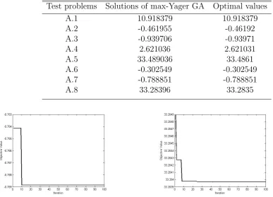
To verify the solutions found by the current method, the optimal solutions of the test problems are also needed. Since S_TP

Y(A, b) is formed as the union of the finite number of convex closed cells (theorem 2), the optimal solutions are also acquired by the following procedure: 1. Computing all the convex cells of the Yager FRE. 2. Searching the optimal solution for each convex cell. 3. Finding the global optimum by comparing these local optimal solutions.

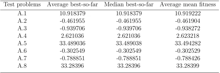
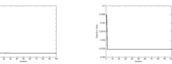
The computational results of the eight test problems are shown in Table 1 and Figures 1-8. In Table 1, the results are averaged over 30 runs and the average best-so-far solution, average mean fitness function and median of the best solution in the last iteration are reported. Table 2 includes the best results found by the current algorithm and the above procedure. According to Table 2, the optimal solutions computed by the algorithm and the optimal solutions obtained by the above procedure match very well. Tables 1 and 2, demonstrate the attractive ability of the algorithm to detect the optimal solutions of problem (1). Also, the good convergence rate of the algorithm could be concluded from Table 1 and figures 1-8.

Table 1: Results of applying the max-Yager GA to the eight test problems. The results have been averaged over 30 runs. Maximum number of iterations=100.

Test problems Average best-so-far Median best-so-far Average mean fitness

A.1 10.918379 10.918379 10.919222

A.2 -0.461955 -0.461955 -0.461904

A.3 -0.939706 -0.939706 -0.938272

A.4 2.621036 2.621036 2.623218

A.5 33.489036 33.489038 33.494282

A.6 -0.302549 -0.302549 -0.302529

A.7 -0.788851 -0.788851 -0.788426

Figure 1: The performance of the proposed algorithm on test problem 1.

Figure 2: The performance of the proposed algorithm on test problem 2.

Figure 3: The performance of the max-Yager GA on test problem 3.

Figure 4: The performance of the max-Yager GA on test problem 2.

Figure 5: The performance of the proposed algorithm on test problem 5.

Table 2: Comparison of the solutions found by the current method and the optimal values of the test problems.

Test problems Solutions of max-Yager GA Optimal values

A.1 10.918379 10.918379

A.2 -0.461955 -0.46192

A.3 -0.939706 -0.93971

A.4 2.621036 2.621031

A.5 33.489036 33.4861

A.6 -0.302549 -0.302549

A.7 -0.788851 -0.788851

A.8 33.28396 33.2835

Figure 7: The performance of the proposed algorithm on test problem 7.

Figure 8: The performance of the proposed algorithm on test problem 8.

5.2

Comparisons with other works

As mentioned before, we can make a comparison between the current algorithm and max-min GA [41]. We apply the current algorithm (modified for the max-minimum t-norm) to the test problems by considering ϕas the minimum t-norm. The results are shown in Table 3 including the optimal objective values found by the current method and max-min GA. As is shown in this table, the current method finds better solutions for test problems 1, 5 and 6, and the same solutions for the other test problems. Table 4 shows that the current algorithm finds the optimal values faster than max-min GA and hence has a higher convergence rate, even for the same solutions. The only exception is test problem 8 in which all the results are the same. In all the cases, results marked with ”*” indicate the better cases.

Conclusion

nec-Table 3: Best results found by the current algorithm and Lu and Fangs method. Test problems Lu and Fang Current algorithm

B.1 8.4296755 8.4296754∗

B.2 -1.3888 -1.3888

B.3 0 0

B.4 5.0909 5.0909

B.5 71.1011 71.0968∗

B.6 -0.3291 -0.4175

B.7 -0.6737 -0.6737∗

B.8 93.9796 93.9796

Table 4: A Comparison between the results found by the current algorithm and Lu and Fangs algorithm.

Test problems Lu and Fang Current algorithm

Average best-so-far 8.4296755 8.4296796∗

B.1 Median best-so-far 8.4296755 8.4296755

Average mean fitness 8.4296755 8.4398745∗ Average best-so-far -1.3888 -1.3888

B.2 Median best-so-far -1.3888 -1.3888

Average mean fitness -1.3877 -1.3886∗

Average best-so-far 0 0

B.3 Median best-so-far 0 0

Average mean fitness 7.1462e-07 0∗

Average best-so-far 5.0909 5.0909

B.4 Median best-so-far 5.0909 5.0909

Average mean fitness 5.0910 5.0908∗ Average best-so-far 71.1011 71.0969∗

B.5 Median best-so-far 71.1011 71.0968∗

Average mean fitness 71.1327 71.1216∗ Average best-so-far -0.3291 -0.4175∗

B.6 Median best-so-far -0.3291 -0.4175∗

Average mean fitness -0.3287 -0.4162∗ Average best-so-far -0.6737 -0.6737

B.7 Median best-so-far -0.6737 -0.6737

Average mean fitness -0.6736 -0.6737∗ Average best-so-far 93.9796 93.9796

B.8 Median best-so-far 93.9796 93.9796

Average mean fitness 93.9796 93.9796

Appendix A

Test Problem A.1:

f(x) = (x1+ 10x2)2+ 5(x3−x4)2+ (x2−2x3)4+ 10(x1−x4)4

bT _{= [0.2077,0.4709,0.8443]}

A= 



0.4302 0.4464 0.0741 0.0751 0.1848 0.1603 0.4628 0.5929 0.9049 0.1707 0.8746 0.4210 



Test Problem A.2:

bT = [0.0871,0.3713,0.2455,0.1801] 

  

0.5801 0.7557 0.0705 0.0568 0.0612 0.6871 0.3217 0.6975 0.6199 0.8560 0.0363 0.5551 0.1511 0.8654 0.1547 0.8343 0.0525 0.1708 0.0591 0.5315



  

Test Problem A.3:

f(x) = x1−x2−ln(1 +x3x4x5)−x6

bT _{= [0.5531,0.2219,0.9524,0.8888]}



  

0.4432 0.4430 0.0774 0.7655 0.2581 0.2074 0.2629 0.0780 0.8817 0.2126 0.5757 0.1161 0.9554 0.9857 0.5055 0.5656 0.1704 0.1256 0.2025 0.1048 0.5135 0.7883 0.8020 0.9774 

  

Test Problem A.4:

f(x) = x1+ 2x2+ 4x5+ex1x4−x6

bT = [0.9296,0.6019,0.1510,0.5746,0.0953]      

0.9486 0.9505 0.1827 0.5498 0.2400 0.0183 0.0787 0.5247 0.8651 0.4489 0.6457 0.1841 0.9116 0.1440 0.0188 0.0400 0.1404 0.0818 0.8890 0.3096 0.4366 0.8204 0.5103 0.3569 0.0567 0.0415 0.0748 0.0888 0.0672 0.1593      

Test Problem A.5:

f(x) =

6

P

k=1

[100(xk+1−x2k)2+ (1−xk)2]

bT _{= [0.3205,0.3143,0.4007,0.7064,0.3223]}

     

0.1588 0.7224 0.1207 0.6127 0.8826 0.7250 0.6135 0.2848 0.9535 0.2324 0.3272 0.9862 0.0513 0.1372 0.0671 0.2631 0.7020 0.9393 0.5195 0.5549 0.5847 0.9175 0.4171 0.7517 0.0661 0.1765 0.7090 0.3740 0.1342 0.8735 0.2747 0.8126 0.3290 0.1664 0.9600      

Test Problem A.6:

f(x) = −0.5(x1x4−x2x3+x2x6−x5x6+x5x4−x6x7)

       

0.1285 0.0451 0.1427 0.1872 0.2295 0.7203 0.6670 0.9561 0.9761 0.2078 0.9746 0.9781 0.4570 0.4021 0.6666 0.8612 0.1218 0.4595 0.8631 0.1837 0.2471 0.5068 0.8627 0.8454 0.4403 0.7161 0.7578 0.9279 0.1450 0.1297 0.1770 0.2023 0.9684 0.6396 0.2200 0.6382 0.3370 0.4653 0.9578 0.6173 0.1641 0.9557        

Test Problem A.7:

f(x) = ex1x2x3x4x5 _−0.5(x3

1+x32 +x36+ 1)2 + 2x7x8

bT _{= [0.2756,0.9283,0.7121,0.0869,0.9084,0.4182]}

       

0.1561 0.1743 0.8339 0.0394 0.6963 0.0332 0.2050 0.2719 0.9810 0.8829 0.4494 0.9293 0.9583 0.9673 0.6076 0.5612 0.1322 0.8624 0.1449 0.3192 0.3495 0.7525 0.7416 0.8593 0.0870 0.9568 0.8332 0.0631 0.0539 0.0090 0.8811 0.0814 0.6490 0.6310 0.2537 0.9922 0.9580 0.9281 0.3140 0.6324 0.1774 0.5941 0.3514 0.2267 0.3360 0.8476 0.1344 0.2842        

Test Problem A.8:

f(x) = (x1−1)2+ (x7−1)2+ 10 7

P

k=1

(10−k)(x2_k−xk+1)2

bT _{= [0.1904,0.3993,0.7326,0.1259,0.5292,0.4251,0.8132]}

         

Appendix B

Test Problem B.1:

f(x) = (x1+ 10x2)2+ 5(x3−x4)2+ (x2−2x3)4+ 10(x1−x4)4

bT _{= [0.2077,0.4709,0.8443]}

A= 



0.4302 0.4464 0.0741 0.0751 0.1848 0.1603 0.4628 0.5929 0.9049 0.1707 0.8746 0.4210 



Test Problem B.2:

f(x) = x1−x2−x3−x1x3+x1x4+x2x3 −x2x4

bT = [0.4228,0.9427,0.9831] 



0.1280 0.7390 0.2852 0.2409 0.9991 0.7011 0.1688 0.9667 0.1711 0.6663 0.9882 0.6981 



Test Problem B.3:

f(x) = x1x2x3x4x5

bT = [0.6714,0.5201,0.1500] 



0.4424 0.3592 0.6834 0.6329 0.9150 0.6878 0.7363 0.7040 0.6869 0.2002 0.6482 0.3947 0.4423 0.0769 0.0175





Test Problem B.4:

f(x) = x1+ 2x2+ 4x5+ex1x4

bT = [0.6855,0.5306,0.5975,0.2992] 

  

0.1025 0.7780 0.3175 0.9357 0.7425 0.0163 0.2634 0.5542 0.4579 0.9213 0.7325 0.2481 0.8753 0.2405 0.4193 0.1260 0.2187 0.6164 0.7639 0.2962



  

Test Problem B.5:

f(x) =

6

P

k=1

[100(xk+1−x2k)2+ (1−xk)2]



  

0.1187 0.4147 0.8051 0.3876 0.3643 0.7031 0.4761 0.8606 0.4514 0.0311 0.5323 0.1964 0.6618 0.2715 0.3826 0.0302 0.7117 0.1784 0.9081 0.1459 0.7896 0.9440 0.8715 0.1265 

  

Test Problem B.6:

f(x) = −0.5(x1x4−x2x3+x2x6−x5x6+x5x4−x6x7)

bT = [0.9879,0.6321,0.8082,0.6650] 

  

0.0832 0.3312 0.4580 0.7001 0.8287 0.9978 0.1876 0.3904 0.4277 0.2302 0.1373 0.4850 0.3495 0.8831 0.2393 0.8619 0.2734 0.8265 0.6598 0.4328 0.9315 0.4863 0.3787 0.6748 0.9301 0.4564 0.5893 0.8943 

  

Test Problem B.7:

f(x) = ex1x2x3x4x5 _−0.5(x3

1+x32 +x36+ 1)2

bT _{= [0.9521,0.0309,0.8627,0.8343,0.6290]}

     

0.9869 0.0805 0.8373 0.1417 0.9988 0.6320 0.0139 0.0169 0.0182 0.4379 0.0295 0.5095 0.2497 0.6914 0.8961 0.3504 0.8225 0.2433 0.9691 0.6170 0.5921 0.4785 0.5994 0.5714 0.6197 0.6298 0.2372 0.5874 0.2560 0.9817      

Test Problem B.8:

f(x) = (x1−1)2+ (x7−1)2+ 10 7

P

k=1

(10−k)(x2

k−xk+1)2

bT = [0.7840,0.4648,0.8864,0.8352,0.9839]      

References

[1] Chang, C. W., Shieh, B. S., Linear optimization problem constrained by fuzzy maxmin relation equations, Information Sciences 234 (2013) 7179.

[2] Chen, L. , Wang, P. P., Fuzzy relation equations (i): the general and specialized solving algorithms, Soft Computing 6 (5) (2002) 428-435.

[3] Chen, L., Wang, P. P., Fuzzy relation equations (ii): the branch-point-solutions and the categorized minimal solutions, Soft Computing 11 (2) (2007) 33-40.

[4] Dempe, S., Ruziyeva, A., On the calculation of a membership function for the solu-tion of a fuzzy linear optimizasolu-tion problem, Fuzzy Sets and Systems 188 (2012) 58-67.

[5] Di Martino, F., Loia, V., Sessa, S., Digital watermarking in coding/decoding processes with fuzzy relation equations, Soft Computing 10(2006) 238-243.

[6] Di Nola, A., Sessa, S., Pedrycz, W., Sanchez, E., Fuzzy relational equations and their applications in knowledge engineering, Dordrecht: Kluwer academic press, 1989.

[7] Dubey, D., Chandra, S., Mehra, A., Fuzzy linear programming under interval uncertainty based on IFS representation, Fuzzy Sets and Systems 188 (2012) 68-87.

[8] Dubois, D., Prade, H., Fundamentals of Fuzzy Sets, Kluwer, Boston, 2000.

[9] Fan, Y. R., Huang, G. H., Yang, A. L., Generalized fuzzy linear programming for decision making under uncertainty: Feasibility of fuzzy solutions and solving approach, Information Sciences 241 (2013) 12-27.

[10] Fang, S. C., Li, G., Solving fuzzy relation equations with a linear objective function, Fuzzy Sets and Systems 103(1999) 107-113.

[12] Freson, S., De Baets, B., De Meyer, H., Linear optimization with bipolar maxmin constraints, Information Sciences 234 (2013) 315.

[13] Ghodousian, A., Khorram, E., An algorithm for optimizing the linear function with fuzzy relation equation constraints regarding max-prod composition, Applied Mathematics and Computation 178 (2006) 502-509.

[14] Ghodousian, A., Optimization of the reducible objective functions with monotone factors subject to FRI constraints defined with continuous t-norms, Archives of Industrial Engineering 1(1) (2018) 1-19.

[15] Ghodousian, A., Babalhavaeji, A., An efficient genetic algorithm for solving nonlinear optimization problems defined with fuzzy relational equations and max-Lukasiewicz composition, Applied Soft Computing 69 (2018) 475492.

[16] Ghodousian, A., Naeeimib, M., Babalhavaeji, A., Nonlinear optimization problem subjected to fuzzy relational equations defined by Dubois-Prade family of t-norms, Computers and Industrial Engineering 119 (2018) 167180.

[17] Ghodousian, A., Raeisian Parvari, M., A modified PSO algorithm for linear optimization problem subject to the generalized fuzzy relational inequalities with fuzzy constraints (FRI-FC), Information Sciences 418419 (2017) 317345.

[18] Ghodousian, A., Zarghani, R., Linear optimization on the intersection of two fuzzy relational inequalities defined with Yager family of t-norms, Journal of Algorithms and Computation 49 (1) (2017) 55 82.

[19] Ghodousian, A., Ahmadi, A., Dehghani, A., Solving a non-convex non-linear optimization problem constrained by fuzzy relational equations and Sugeno-Weber family of t-norms, Journal of Algorithms and Computation 49 (2) (2017) 63 101.

[20] Ghodousian, A., Khorram, E., Fuzzy linear optimization in the presence of the fuzzy relation inequality constraints with max-min composition, Information Sciences 178 (2008) 501-519.

[22] Ghodousian, A., Khorram, E., Solving a linear programming problem with the convex combination of the max-min and the max-average fuzzy relation equations, Applied Mathematics and computation 180 (2006) 411-418.

[23] Guo, F.F., Pang, L. P., Meng, D., Xia, Z. Q., An algorithm for solving optimization problems with fuzzy relational inequality constraints, Information Sciences 252 ( 2013) 20-31.

[24] Guo, F. F., Xia, Z. Q., An algorithm for solving optimization problems with one linear objective function and finitely many constraints of fuzzy relation inequalities, Fuzzy Optimization and Decision Making 5(2006) 33-47.

[25] Guu, S. M., Wu, Y. K., Minimizing a linear objective function under a max-t-norm fuzzy relational equation constraint, Fuzzy Sets and Systems 161 (2010) 285-297.

[26] Guu, S. M., Wu, Y. K., Minimizing a linear objective function with fuzzy relation equation constraints, Fuzzy Optimization and Decision Making 12 (2002) 1568-4539.

[27] Guu, S. M., Wu, Y. K., Minimizing an linear objective function under a max-t-norm fuzzy relational equation constraint, Fuzzy Sets and Systems 161 (2010) 285-297.

[28] Han, S. C., Li, H. X., Notes on pseudo-t-norms and implication operators on a complete Brouwerian lattice and pseudo-t-norms and implication operators: direct products and direct product decompositions, Fuzzy Sets and Systems 153(2005) 289-294.

[29] Hock, W., Schittkowski, K., Test examples for nonlinear programming codes Lecture Notes in Economics and Mathematical Systems, vol. 187, Springer, New York, 1981.

[30] Khorram, E., Ghodousian, A., Linear objective function optimization with fuzzy relation equation constraints regarding max-av composition, Applied Mathematics and Computation 173 (2006) 872-886.

[32] Lee, H. C., Guu, S. M., On the optimal three-tier multimedia streaming services, Fuzzy Optimization and Decision Making 2(1) (2002) 31-39.

[33] Li, P. K., Fang, S. C., On the resolution and optimization of a system of fuzzy relational equations with sup-t composition, Fuzzy Optimization and Decision Making 7 (2008) 169-214.

[34] Li, P., Liu, Y., Linear optimization with bipolar fuzzy relational equation constraints using lukasiewicz triangular norm, Soft Computing 18 (2014) 1399-1404.

[35] Li, P., Fang, S. C., A survey on fuzzy relational equations, part i: classification and solvability, Fuzzy Optimization and Decision Making 8 (2009) 179-229.

[36] Lin, J. L., On the relation between fuzzy max-archimedean t-norm relational equations and the covering problem, Fuzzy Sets and Systems 160 (2009) 2328-2344.

[37] Lin, J. L., Wu, Y. K., Guu, S. M., On fuzzy relational equations and the covering problem, Information Sciences 181 (2011) 2951-2963.

[38] Liu, C.C., Lur, Y.Y., Wu, Y. K., Linear optimization of bipolar fuzzy relational equations with max-ukasiewicz composition, Information Sciences 360 (2016) 149162.

[39] Loetamonphong, J., Fang, S. C., Optimization of fuzzy relation equations with max-product composition, Fuzzy Sets and Systems 118 (2001) 509-517.

[40] Loia, V., Sessa, S., Fuzzy relation equations for coding/decoding processes of images and videos, Information Sciences 171(2005) 145-172.

[41] Lu, J., Fang, S. C., Solving nonlinear optimization problems with fuzzy relation equations constraints, Fuzzy Sets and Systems 119(2001) 1-20.

[43] Nayeed, F., Hanmandlu, M., Three information set-based feature types for the recognition of faces / Signal, Image and Video Processing 10(2) (2016) 327-334.

[44] Nobuhara, H., Hirota, K., Pedrycz, W., Relational image compression: optimizations through the design of fuzzy coders and YUV colors space, Soft Computing 9 (2005) 471-479.

[45] Nobuhara, H., Hirota, K., Di Martino, F., Pedrycz, W., Sessa, S., Fuzzy relation equations for compression/decompression processes of color images in the RGB and YUV color spaces, Fuzzy Optimization and Decision Making 4 (2005) 235-246.

[46] Oantarci, S., Vahaplar, A., Kinay, A. O., Nasibov, E., Influence of T-norm and T-conorm operators in Fuzzy ID3 algorithm , IEEE International Conference on Fuzzy Systems, 2015, Istanbul, Turkey.

[47] Oastro-Company, F., Tirado, P., On Yager and Hamacher t-Norms and Fuzzy Metric Spaces , International Journal of Intelligent Systems 29 (12) (2014) 1173-1180.

[48] Pedrycz, W., Vasilakos, A. V., Modularization of fuzzy relational equations, Soft Computing 6(2002) 3-37.

[49] Peeva, K., Resolution of fuzzy relational equations-methods, algorithm and software with applications, Information Sciences 234 (2013) 44-63.

[50] Perfilieva, I., Fuzzy function as an approximate solution to a system of fuzzy relation equations, Fuzzy Sets and Systems 147(2004) 363-383.

[51] Perfilieva, I., Novak, V., System of fuzzy relation equations model of IF-THEN rules, Information Sciences 177 (16) (2007) 3218-3227.

[52] Perfilieva, I., Finitary solvability conditions for systems of fuzzy relation equations, Information Sciences 234 (2013)29-43.

[54] Sanchez, E., Resolution of composite fuzzy relation equations, Inf. Control 30(1976) 38-48.

[55] Shieh, B. S., Infinite fuzzy relation equations with continuous t-norms, Information Sciences 178 (2008) 1961-1967.

[56] Shieh, B. S., Minimizing a linear objective function under a fuzzy max-t-norm relation equation constraint, Information Sciences 181 (2011) 832-841.

[57] Sun, F., Conditions for the existence of the least solution and minimal solutions to fuzzy relation equations over complete Brouwerian lattices, Information Sciences 205 (2012) 86-92.

[58] Sun, F., Wang, X. P., Qu, x. B., Minimal join decompositions and their applications to fuzzy relation equations over complete Brouwerian lattices, Information Sciences 224 (2013) 143-151.

[59] Wang, S., Fang, S. C., Nuttle, H. L. W., Solution sets of interval-valued fuzzy relational equations, Fuzzy Optimization and Decision Making 2 (1)(2003) 41-60.

[60] Wang, P. Z., Latticized linear programming and fuzzy relation inequalities, Journal of Mathematical Analysis and Applications 159(1991) 72-87.

[61] Wu, Y. K., Guu, S. M., A note on fuzzy relation programming problems with max-strict-t-norm composition, Fuzzy Optimization and Decision Making 3(2004) 271-278.

[62] Wu, Y. K., Guu, S. M., An efficient procedure for solving a fuzzy relation equation with max-Archimedean t-norm composition, IEEE Transactions on Fuzzy Systems 16 (2008) 73-84.

[63] Wu, Y. K., Optimization of fuzzy relational equations with max-av composition, Information Sciences 177 (2007) 4216-4229.

[65] Wu, Y. K., Guu, S. M., Liu, J. Y., Reducing the search space of a linear fractional programming problem under fuzzy relational equations with max-Archimedean t-norm composition, Fuzzy Sets and Systems 159 (2008) 3347-3359.

[66] Xiong, Q.Q., Wang, X. P., Fuzzy relational equations on complete Brouwerian lattices, Information Sciences 193 (2012) 141-152.

[67] Xiong, Q. Q., Wang, X. P., Some properties of sup-min fuzzy relational equations on infinite domains, Fuzzy Sets and Systems 151(2005) 393-402.

[68] Yang, X. P., Zhou, X. G., Cao, B. Y., Latticized linear programming subject to max-product fuzzy relation inequalities with application in wireless communication, Information Sciences 358359 (2016) 4455.

[69] Yang, S. J., An algorithm for minimizing a linear objective function subject to the fuzzy relation inequalities with addition-min composition, Fuzzy Sets and Systems 255 (2014) 41-51.