Application of Machine Learning Techniques for Real-time Classification of Sensor Array Data

(1)

University of New Orleans University of New Orleans

ScholarWorks@UNO

University of New Orleans Theses and

Dissertations Dissertations and Theses

5-15-2009

Application of Machine Learning Techniques for Real-time

Classification of Sensor Array Data

Sichu Li

University of New Orleans

Follow this and additional works at: https://scholarworks.uno.edu/td

Recommended Citation Recommended Citation

Li, Sichu, "Application of Machine Learning Techniques for Real-time Classification of Sensor Array Data" (2009). University of New Orleans Theses and Dissertations. 913.

https://scholarworks.uno.edu/td/913

This Thesis is protected by copyright and/or related rights. It has been brought to you by ScholarWorks@UNO with permission from the rights-holder(s). You are free to use this Thesis in any way that is permitted by the copyright and related rights legislation that applies to your use. For other uses you need to obtain permission from the rights-holder(s) directly, unless additional rights are indicated by a Creative Commons license in the record and/or on the work itself.

(2)

Application of Machine Learning Techniques for Real-time Classification of Sensor Array Data

A Thesis

Submitted to the Graduate Faculty of the University of New Orleans in partial fulfillment of the requirements for the degree of

Master of Science in

Computer Science

by

Sichu Li

Ph.D. University of New Orleans, 1997

(3)

ii

(4)

iii

To my husband Peter Rochford, my children Ashley and Kevin Rochford,

(5)

iv

Acknowledgement

I would like to express my heartfelt appreciation to my thesis advisor Dr. Dongxiao Zhu

for his suggestion of investigating machine learning techniques for the classification of sensor

array data for my thesis topic. The author really benefited from his knowledge, advice and

direction during the preparation of this thesis.

I also wish to express my appreciation to my thesis committee, Drs. Christopher Summa

and Christopher Taylor, for their time in reviewing and providing constructive comments on the

thesis.

In addition, I express my thanks to all of the members of the faculty in the Computer

Science Department at the University of New Orleans, for their teaching in the various courses I

took, where I learned and acquired my knowledge in computer science.

Finally, I would like to thank my family for their strong support during the preparation of

this thesis. Without the endless encouragement from my husband, Dr. Peter Rochford, and

constant inspiration from my lovely children, Ashley and Kevin Rochford, this thesis would

(6)

v

List of Figures

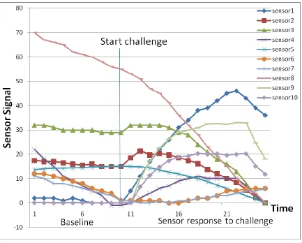
Figure 1: Simulated sensor signal as a function of time for a 10-channel sensor array ... 9

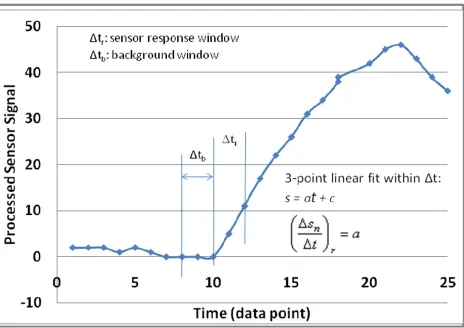
Figure 2: Illustration of first derivative calculation within a sensor response or background window. ... 10

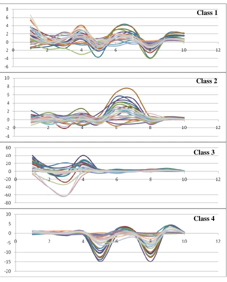
Figure 3. Predictor values vs. predictor number (sensor channel). ... 12

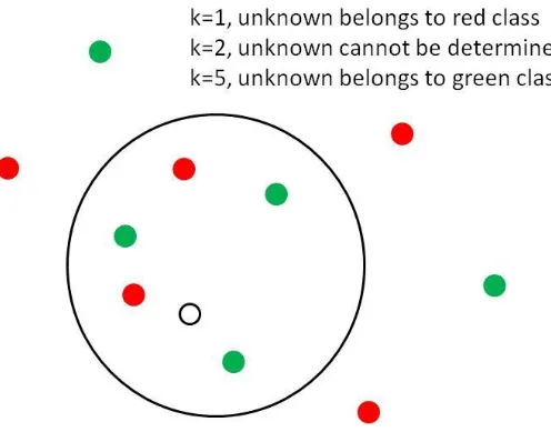
Figure 4: A simple KNN classification for an unknown indicated by the empty circle. ... 16

Figure 5: Overall success rate vs. k value obtained from KNN 10-fold ... 20

Figure 6. A simple linear SVM classification. ... 22

Figure 7. An example SVM classification. ... 23

Figure 8. Kernel transformation in SVM. ... 24

Figure 9. CART decision tree for multi-channel sensor data. ... 33

Figure 10. Variation of cross validation error with number of principal components for the 4 classes. ... 47

Figure 11. Prediction success rates for the testing dataset using KNN method. ... 52

Figure 12. Dendrogram of the training dataset. ... 53

Figure 13. Prediction success rates for the testing dataset using SVM method. ... 55

Figure 14. Classification success rates for the testing dataset using CART method. ... 57

Figure 15. Classification success rates using Naïve Bayes Classifer with both linear and quadratic ... 61

Figure 16. Predicted Y-block values for each class. ... 64

Figure 17: Prediction success rates for the testing dataset based on maximum Y-Block value from PCR method. ... 67

(9)

viii

List of Tables

Table 1: KNN 10-fold cross-validation results. ... 19

Table 2: Percentage success rates from KNN 10-fold cross-validation. ... 20

Table 3. Initial and optimal parameters for the SVM model. ... 27

Table 4: CART self-prediction results. ... 34

Table 5: Percentage success rates from CART self-prediction. ... 34

Table 6: Prediction results for the testing dataset using KNN method. ... 52

Table 7: Prediction results for the testing dataset using SVM method. ... 55

Table 8: Prediction results for the testing dataset using CART method. ... 57

Table 9. Dependence of classification success rate on the number of trees used in Random Forest method... 59

Table 10: Prediction results for the testing dataset using RF method with 50 trees. ... 59

Table 11: Prediction results for the testing dataset using Naive Bayes method. ... 61

Table 12: Prediction results for the testing dataset using PCR method. ... 65

Table 13: Classification of unknown samples based on their maximum Y-block value. ... 66

(10)

ix

Abstract

There is a significant need to identify approaches for classifying chemical sensor array

data with high success rates that would enhance sensor detection capabilities. The present study

attempts to fill this need by investigating six machine learning methods to classify a dataset

collected using a chemical sensor array: K-Nearest Neighbor (KNN), Support Vector Machine

(SVM), Classification and Regression Trees (CART), Random Forest (RF), Naïve Bayes

Classifier (NB), and Principal Component Regression (PCR). A total of 10 predictors that are

associated with the response from 10 sensor channels are used to train and test the classifiers. A

training dataset of 4 classes containing 136 samples is used to build the classifiers, and a dataset

of 4 classes with 56 samples is used for testing. The results generated with the six different

methods are compared and discussed. The RF, CART, and KNN are found to have success rates

greater than 90%, and to outperform the other methods.

(11)

1

Chapter 1

(12)

2

An electronic nose (E-nose) is an instrument that is designed to mimic the function of the

natural nose. By definition, it not only detects but also discriminates among complex chemical

vapors [1], with a sensor array typically consisting of a group of non-specific chemical sensors

that respond to chemical vapors. The detection, classification, and identification of a particular

chemical is based on a unique combinatory response pattern from all sensors rather than the

response pattern from a particular sensor. In addition to the sensor substrates, the response

pattern recognition algorithm is a key component in an E-nose system that determines how well

the E-nose identifies the chemicals. Improvements in the response pattern recognition algorithm

can therefore provide major advances in the detection capabilities of the instrument, and drives

the need to identify approaches for classifying chemical sensor array data with high success

rates. In this study, we attempt to fill this need by investigating the feasibility of using machine

learning techniques to classify chemical sensor array data for detection of different classes of

chemical subjects.

In a chemical system, classes may differ for many reasons, including variations in sample

preparation, differences in chemical compound type (aromatic, aliphatic, carbonyl, etc.), or

variations in process state (startup, normal, particular faults, etc.). In this study, classes are

referred to by chemical compound type (carbonyl, amine, carboxyl, and aromatic structure).

Almost all chemical systems are complex because different chemical components are typically

related to each other in a certain way. It is possible that all channels (sensors) could react to an

individual chemical, thereby making classification of the response of a chemical sensor array

non-trivial, and requiring that the classification be based on a combination of responses rather

(13)

3

A variety of methods have been developed for classifying samples based on the measured

sensor response [2]. These methods fall into the two general categories of cluster analysis or

unsupervised pattern recognition, and classification or supervised pattern recognition, where the

former attempts to identify groups or classes without using pre-established class memberships,

and the latter uses known class memberships. Classification of new unknown samples can be

accomplished manually using unsupervised methods, or automatically using supervised

techniques. Since our objective is to develop a classification algorithm for a real-time sensor

array, the supervised approach is of interest because it can be implemented to provide

classification results online.

To classify multi-channel sensor data, typically a Principal Component Analysis

(PCA)-based method is used to decompose the covariance matrix among different sensor channels into

orthogonal Principal Components (PCs), and then a certain discriminating approach is used for

classification. Chemometric methods have also been widely exploited to classify chemicals for

sensor arrays composed of multiple channels (a group of sensors) [3, 4]. Typical applications of

chemometric methods employ the development of quantitative structure activity relationships or

the evaluation of analytical–chemical data to perform the classification. In addition, a variety of

statistical methods have been adapted into chemometrics for classification to solve

chemical-related problems such as the K-nearest neighbor, PCA, and the Partial Least Squares

Discriminant Analysis (PLS-DA) [5, 6]. The success rates using these approaches are rarely high

enough to satisfy instrument detection requirements, and the classification model needs to be

recalibrated often. This drives us to explore alternative approaches to improve classification.

In this study, we explore using supervised machine learning techniques to improve

(14)

4

and practical technique for discovering relations and extracting knowledge because they are able

to map inputs to desired outputs in a robust manner. Since detection targets are known in most

cases, we can obtain a training dataset by testing the sensor array with standard chemical

samples. In addition, it is possible to collect the training dataset under a variety of operational

conditions to ensure that the dataset is representative. A variety of machine learning methods are

considered here to evaluate their potential benefits for classification of multi-channel sensor data

because the distinct mechanisms each employs.

The objective of this study is to compare the predictive accuracy of six of the more

popular classifiers used in the scientific community on a multi-channel chemical sensor array

dataset: K-Nearest Neighbor (KNN), Support Vector machine (SVM), Classification and

Regression Trees (CART), Random Forests (RF), Naïve Bayes Classifier (NB), and Principal

Component Regression (PCR). The sensor dataset is constructed from 4 classes of 48 data

samples, with 34 samples selected from each class to form a training dataset of 136 (34×4) data

samples. The remaining samples are used to form a testing dataset of 56 (14×4) data samples.

Since the individual sensors (channels) of the sensor array respond to chemical stimuli

differently in their signal change (increase or decrease, intensity of the change), a predictor is

assigned to each channel to reflect its contribution to a combined response pattern of the sensor

array. Therefore, 10 predictors (variables) are used in training and testing the classifiers.

In the remainder of this thesis, we first describe the nature of the dataset and the features

captured within it (Chapter 2). We then present six classifier methods (Chapters 3 to 8),

providing a brief description of each method, the training of each model, and its validation and

testing. Finally, we present and discuss the prediction results generated using each classifier

(15)

5

Chapter 2

(16)

6

The multi-channel sensor dataset used for this study was collected by challenging a

sensor array with 4 groups of chemicals with different molecular structures (carbonyl, amine,

carboxyl, and aromatic structure). Each data sample is a combined response from 10 different

types of chemical sensors on a sensor array, where each chemical sensor is referred to as a sensor

channel. Each group of chemicals was tested for three concentration levels (high, medium, and

low), and the data collected from challenges with the same group of chemicals forms a class. The

steps carried out to construct the 4 classes within the dataset used for this study are described

next.

2.1 Feature Vector Extraction

A response to a chemical stimulus from a sensor channel is triggered by a chemical

reaction between the sensing element and the chemical. The reaction results in a change in a

particular property (ΔP), and this change typically depends on the chemical concentration (C).

The relationship between ΔP and C can be non-linear over a long time window due to the change

in sensor sensitivity over time. However, for online classification, the time period over which the

sensor data is collected is invariably short. For example, for this sensor array a time window

covered by 3 data points after the start of sampling. The sensor response is typically assumed to

have a linear relationship with the concentration of the collected chemical, as expressed by the

relation

ΔP= α C

where α is a parameter that is highly associated with the sensor channel behavior. For a single

sensor channel, the sensitivity and chemical collection efficiency determine its parameter α.

Therefore, α can be used as a marker to indicate the behavior of each sensor channel.

(17)

7

of a chemical stimulus, ΔP can then be usedto indicate the sensor channel behavior. The

question is how to express the property change ΔP. Since every measured signal includes not

only a signal of the property of interest but also contributions from the background (due to

certain cross-reactions with chemicals residing in the environment) and some system noise, ΔP

must be calculated in a manner to minimize such effects. To reduce noise, ΔP is evaluated as a

rate of change over a given time window (ΔP/Δt)r. To remove the background contribution, the

rate of change (ΔP/Δt)b is calculated within a time window just before the sensor experiences the chemical stimuli, and this value is then subtracted from the rate of change ((ΔP/Δt)r within

the same length time window immediately after. Since the sensor array was developed to meet a

system requirement of classifying the chemical stimuli within a short time window, for which its

sampling capability could only provide 3 data points, the time window used to evaluate the rate

of change in sensor signal was limited to 3 data points.

Figure 1 shows an example of simulated data from the 10 sensor channels before and

after a chemical challenge occurs at the point indicated by “Start challenge”. The data reveals

that each sensor channel responds to the challenge with a different rate of signal change. For

some sensor channels there is a noticeable baseline drifting prior to the challenge, while for some

sensor channels the response is more rapid than others. To adequately capture this signal change

over time, a rate is calculated for each sensor channel s_n as the difference between the

instantaneous rate and a baseline signal drift rate

b n

r n n

t s t

(18)

8

where n is the sensor channel number (1 to 10). As shown in Figure 2,

r n t s

is the signal

change rate after the start of the challenge, and

b n t s

is the baseline signal drifting rate

immediately before challenge. The time window (Δ t) used for calculating the signal change rate

is a 3 data point period for the reason given above. The actual values of the signal change rate are

evaluated from a least-squares fit of the 3 data point values. The resultant linear function is

s

= a

t

+ c

from which one obtains the signal change rate a t s r n _and a t s b

n _{for data points in the}

r

t and t_b time windows, respectively. These signal change rates for the sensor channels are

used to define 10 feature element values (predictors) that form the training and testing datasets to

which the classification models described further below are applied. For the sensor channels that

respond to the challenge more quickly, the time window is from the first to third data point

reading after a challenge. For those that have a slower response, Δt starts from the second to

fourth data reading after a challenge, i.e. one data point reading delay. Thus each data sample is

converted to a vector:

= (

x

1

, x

2

, x

3

, … x

10

)

(19)

9

Figure 1: Simulated sensor signal as a function of time for a 10-channel sensor array

(20)

10

(21)

11

Plots of predictor value versus predictor number (sensor channel number) for each

training data sample for 4 classes are shown in Figure 3. From the general variation in the curves

it can be seen that the features of classes 3 and 4 are more distinct than the others, while the

features of classes 1 and 2 exhibit certain cross-reactivity between each other and with class 3.

While quantities other than sensor signal change rate might be used for the feature vector, as

stated above, it is employed here because it provides the most direct indication of sensor

behavior that can be employed to reduce noise. Moreover, a least-squares fit provides the best

(22)

12

Figure 3. Predictor values vs. predictor number (sensor channel).

Class 4

Class 3

Class 2

Class 1

(23)

13

2.2 Training and Testing Dataset

In this study there are 4 classes of 48 data samples, with 34 samples randomly selected

from each class to form a training dataset of 136 (34×4) data samples. The remaining samples

are used to form a testing dataset of 56 (14×4) data samples. Because the sensor behavior

depends on environmental operational conditions such as temperature and humidity, and the 48

data samples in each class were collected from 4 trials, each with different operational

conditions, the 34 data samples in each class were randomly selected from the 48 data samples to

ensure the training dataset captured the variability in conditions. Furthermore, since the 48 data

samples in each class have equal numbers of 16 samples with respect to high, medium, and low

challenge concentrations, the number of data samples randomly selected for each of the three

concentration levels is nearly equal in both the training and testing datasets. This ensures a fair

representation from each concentration level within a class. Figure 3 provides predictor values

vs. predictor numbers for the training dataset.

2.3 Dataset for Cross-validation

In constructing some machine learning models for prediction, we performed a cross

validation to obtain the optimal model parameter values, e.g. K value in KNN, Cross validation

is a method to estimate the error rate in an efficient and unbiased way. The procedure works as

follows: the dataset is first divided into k sub-samples (k ≤ 10) (in our experiments k = 10 for

each class). A single sub-sample is then chosen as testing data, and the remaining (k – 1)

subsamples are used as training data. The procedure is repeated k (10) times, in which each of

the k subsamples is used exactly once as the testing data. All testing results, 34 predictions for

(24)

14

Chapter 3

(25)

15

3.1 Method

The k-nearest neighbor (KNN) method [7] is one of the most popular algorithms to

implement because it is simple, powerful, yet model free. It functions on the intuitive idea that

close objects are more likely to be in the same class. The method finds k known observations x

in a training dataset that are closest to the unknown test observation y to predict the classification

of the latter (Figure 4), where k is a positive integer that is typically small. The class of y is

predicted based on the majority vote of the classes of these k neighbors, hence the name k

-Nearest Neighbor. In the simplest case when k = 1 (nearest neighbor), y is simply assigned to the

class of its nearest neighbor x. Closeness implies a metric for the distance D(x,y) between x and

y that must be defined, such that the smaller the distance, the closer x is to y. One of the most

popular choices for the metric is Euclidean distance, while other choices are Euclidean squared,

City-block, and Chebychev:

|) max(| ) ( ) ( ) ( ) , ( 2 2 y x y x abs y x y x y x D Chebychev block City squared Euclidian Euclidian

where the difference between x and y is in terms of a difference in vectors. The KNN method

relies on having a set of observations for which the outcome is known, i.e. a set of independent

values labeled by a set of dependent outcomes. (The independent and dependent variables can be

either continuous or categorical). For continuous dependent variables, the task is regression;

otherwise it is a classification. For the application being investigated here the KNN method is

(26)

16

Figure 4: A simple KNN classification for an unknown indicated by the empty circle.

The choice of k is essential in building the KNN model as it can strongly influence the

quality of predictions. One appropriate way to look at the number of nearest neighbors k is to

think of it as a smoothing parameter. For any given problem, a small value of k will lead to a

large variance in predictions. Alternatively, setting k to a large value may lead to a large model

bias. Thus, k should be set to a value large enough to minimize the probability of

misclassification and small enough (with respect to the number of observations in the training

dataset ) so that the k nearest observations are close enough to the unknown test observation .

Thus, like any smoothing parameter, there is an optimal value for k that achieves the right trade

off between the bias and the variance of the model.

The value of k can be found using a cross-validation algorithm. It entails dividing the

data sample into a number of sub-samples. For a fixed value of k, the KNN model is applied to

make predictions on one sub-sample (using the remaining subsamples as the prototype examples)

(27)

17

(the percentage of correctly classified observations). This process is then successively applied to

all possible choices of sub-samples. After cycling through all the sub-samples, the computed

errors are averaged to determine how well the model predicts the known test observations. The

above steps are then repeated for various k and the value achieving the lowest error (or the

highest classification accuracy) is then selected as the optimal value for k (optimal in a

cross-validation sense). Note that cross-cross-validation is computationally expensive.

3.2 Training

The PLS_Toolbox (Version 4.2) developed by Eigenvector Research Inc. for multivariate

analysis of chemometrics within the Matlab™ computational environment [8] was used to

perform the KNN training. The “knn” function within PLS_Toolbox was employed for both

cross-validation and the predicted classification. The feature vectors in the training and testing

datasets were supplied to the function as a N×10 float array of data, where each row represented

a single feature vector. The class values for both datasets were provided as a N×1 integer array,

with each row being the class value (1 through 4) of the corresponding feature vector in the

N×10 float array of data. Autoscaling was applied to both the training and testing feature vectors

by centering the columns of the feature vectors to zero mean and scaling them to unit variance,

and the closest neighbor was assigned to the predicted class if there was no majority vote

amongst the nearest neighbors.

3.3 Validation

The cross-validation to determine the optimal choice of k nearest neighbors was

accomplished by excluding a subset of the training dataset of N (N = 10 in this study) subsets of

(28)

18

the constructed model to predict the class of the excluded vector. This process was repeated for

all feature vectors in the training set, accumulating statistics on the number of successful

predictions by comparing the predicted class of the excluded vector against its known class. The

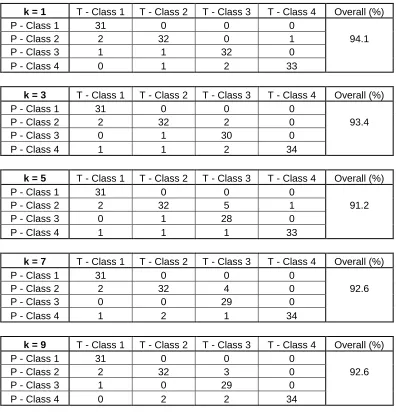
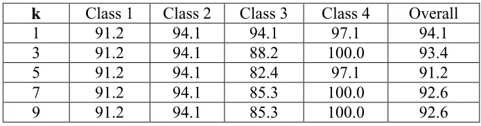
cross validation was performed for odd values k = 1 through 9. The results are listed in Table 1,

and the success rates were calculated and shown in Table 2. These results indicate the

constructed model has a very high performance for prediction within the training dataset, with a

constant success rate for the class 1 and 2 features, small variability for class 4, and moderate

variability for class 3. As shown in Figure 5, the highest success rate is obtained when using k=1,

i.e. the nearest neighbor. The average success rate for all classes decreases for k=1 to 5 and then

slightly increases to a constant value thereafter, indicating that increasing the number of nearest

neighbors saturates the voted closest class beyond k =7. Therefore, k=1 is used for the KNN

model prediction of the sensor array data.

3.4 Testing

The KNN method was tested by using the “knn” function to build the model with the

training dataset and k=1 as input along with the option of autoscaling. The results are shown and

(29)

19

Table 1: KNN 10-fold cross-validation results.

k = 1 T - Class 1 T - Class 2 T - Class 3 T - Class 4 Overall (%)

P - Class 1 31 0 0 0

P - Class 2 2 32 0 1 94.1

P - Class 3 1 1 32 0

P - Class 4 0 1 2 33

P - Class 1 31 0 0 0

P - Class 2 2 32 2 0 93.4

P - Class 3 0 1 30 0

P - Class 4 1 1 2 34

P - Class 1 31 0 0 0

P - Class 2 2 32 5 1 91.2

P - Class 3 0 1 28 0

P - Class 4 1 1 1 33

P - Class 1 31 0 0 0

P - Class 2 2 32 4 0 92.6

P - Class 3 0 0 29 0

P - Class 4 1 2 1 34

P - Class 1 31 0 0 0

P - Class 2 2 32 3 0 92.6

P - Class 3 1 0 29 0

P - Class 4 0 2 2 34

(30)

20

Table 2: Percentage success rates from KNN 10-fold cross-validation.

k Class 1 Class 2 Class 3 Class 4 Overall

1 91.2 94.1 94.1 97.1 94.1

3 91.2 94.1 88.2 100.0 93.4

5 91.2 94.1 82.4 97.1 91.2

7 91.2 94.1 85.3 100.0 92.6

9 91.2 94.1 85.3 100.0 92.6

Figure 5: Overall success rate vs. k value obtained from KNN 10-fold

(31)

21

Chapter 4

(32)

22

4.1 Method

Support Vector Machines (SVM) is a powerful technique for classification problems [9,

10], and is one of the most popular classifiers these days. It is based on the concept of decision

planes that define decision boundaries separating sets of objects having different class

memberships. It is primarily a classifier method that performs classification tasks by constructing

hyperplanes in a multidimensional space that separates cases of different class labels. SVM

supports both regression and classification tasks and can handle multiple continuous and

categorical variables. Because of the nature of the feature space in which these boundaries are

found, SVMs can exhibit a large degree of flexibility in handling classification and regression

tasks of varied complexity.

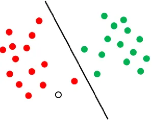
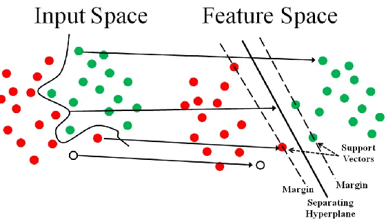
The goal of SVM is to construct a separating hyperplane that is maximally distant from

different classes of the training data. To illustrate, an example is shown in Figure 6 of objects

that belong to either class GREEN or RED. The separating line defines a boundary on the right

side of which all objects are GREEN and to the left of which all objects are RED. Any new

object (white circle) falling to the right is labeled, i.e., classified, as GREEN (or classified as

RED should it fall to the left of the separating line).

(33)

23

This is a classic example of a linear classifier that separates a set of objects into their

respective groups (GREEN and RED in this case) with a line. However, most classification tasks

are not so simple, and require more complex discriminating functions to make an optimal

separation, i.e., correctly classify new objects on the basis of the examples that are available.

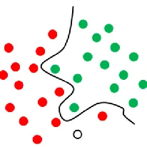
This is illustrated by the example in Figure 7 where a full separation of the GREEN and RED

objects would require a curve.

Figure 7. An example SVM classification.

The basic idea behind SVM is to rearrange the original objects using a set of

mathematical functions (kernels) into a linearly separable arrangement as illustrated Figure 8. As

a result of the transformation, the task of separation is reduced to finding an optimal line that can

separate the GREEN and the RED objects on the right side of Figure 8 rather than constructing

the complex curve as appears on the left side. As shown in Figure 8 the points lying on the

boundaries are called support vectors, and the middle of the margin is the optimal separating

hyperplane that maximizes the margin of separation. Classification tasks based on drawing

separating lines to distinguish between objects of different class memberships are referred to as

(34)

24

Figure 8. Kernel transformation in SVM.

For categorical variables a dummy variable is created with case values of either 0 or 1.

Thus, a categorical dependent variable consisting of three levels, say (A, B, C), is represented by

a set of three dummy variables:

} 1 0 0 { : }, 0 1 0 { : }, 0 0 1 {

: B C

A

To construct an optimal hyperplane, SVM employs an iterative training algorithm, which

is used to minimize an error function. There are two distinct groups for classification SVM

models according to the form of the error function.

4.1.1 Classification SVM Type 1

For this type of SVM, training involves the minimization of the error function

N i i T C w w 1 2 1 ,

subject to the constraints

1 ) ) (

(w x b

(35)

25

where C is the capacity constant, w is the vector of coefficients, b a constant and the _i are

parameters for handling non-separable data (inputs). The index i labels the N training cases. Note

that y 1 is the class labels and x is the vector of independent variables. The kernel is used

to transform data from the input (independent) to the feature space (see below). The vector w is

normal and perpendicular to the hyperplane. The parameter b/w determines the offset of the

hyperplane from the origin along the normal vector w. It should be noted that the larger the C,

the more the error is penalized. Thus, C should be chosen with care to avoid over fitting.

4.1.2 Classification SVM Type 2

In contrast to Classification SVM Type 1, the Classification SVM Type 2 model

minimizes the error function

N i i T N w w 1 1 2 1 ,

subject to the constraints

i T

b x w ( ) )

(  and _i 0,i 1,,N,and 0.

4.1.3 Kernel functions

There are a number of kernels that can be used, and these include linear, polynomial,

radial basis function (RBF), and sigmoid:

) tanh( 0 ), / exp( ) ( ) ,

( 2 ₂ ₂

(36)

26

The RBF is by far the most popular choice of kernel types used in SVMs. This is mainly

because of their localized and finite responses across the entire range of the real x-axis. Although

SVMs are very powerful and commonly used in classification, they suffer from several

drawbacks. They require high computations to train the data, and they are sensitive to noisy data

thereby being prone to over fitting.

4.2 Training

The Least Squares Support Vector Machine (LS-SVM) toolbox (Version 1.5) provided

by the Katholieke Universiteit Leuven, Belgium [11-13] was used to build a SVM for the

multi-sensor data. To set up the model for classification, the class values of the training dataset were

first organized into a N×4 Y-block with values of 0 or 1, where the first column indicated the

feature vectors in the N×10 float array belonging to class 1, the second column to class 2, etc. A

value of 1 was used to identify the given feature vector as belonging to the class, and a value of 0

if it was not a member of the class. A RBF was chosen as the kernel for the model because of its

localized and finite response across the entire range of the real x-axis. The LS-SVM toolbox uses

Type 1 classification by default.

4.3 Validation

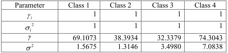
The “tunelssvm” function was used to determine the optimal hyperparameters for the

model: the values for the regularization parameter ( ), determining the trade-off between the

fitting error minimization and smoothness, and the RBF kernel parameter ( 2_{). The tuning was}

performed for classification (“type” of “c”) using the training dataset, with independent and

2_{parameter values for each of the 4 columns of the Y-block. The tuning function uses L-fold}

(37)

27

this type of cross validation the data is permutated randomly once, then divided into L (by

default 10) disjoined sets. In the i-th (i=1, ..., L) iteration, the i-th set is used to estimate the

performance (validation set) of the model trained on the other L-1 sets (training set). In the final

step the L different estimates of the performance are averaged (mean). The assumption is made

that the input data are distributed independent and identically over the input space. The tuning

function yielded the optimal values shown in Table 3 for the indicated initial values of _i and

2

i . The “trainlssvm” function was then employed to train the SVM for classification using the

training dataset. The support values (α) and bias (b) obtained were then used with the

“simlssvm” function to predict the class values for the feature vectors of the training dataset.

Table 3. Initial and optimal parameters for the SVM model. Parameter Class 1 Class 2 Class 3 Class 4

i 1 1 1 1

2

i 1 1 1 1

69.1073 38.3934 32.3379 74.3043

2 1.5675 1.3146 3.4980 7.0838

4.4 Testing

The SVM model was tested by using the “simlssvm” function to make predictions for the

testing dataset. The training dataset was input along with the optimal and 2_parameter

values, specification of a RBF kernel, the support values (α) and bias (b) obtained from the

tuning, and the feature vectors of the testing dataset. The results obtained are shown and

(38)

28

Chapter 5

(39)

29

5.1 Method

CART is a well-known method for constructing a classification tree from data [14]. It is a

model that describes the conditional distribution of y given x. It consists of two components: a

tree T with b terminal nodes, and a parameter vector p= (p1, p2, … , pb) where pi is associated with

the ith terminal node. Each terminal node of the tree corresponds to a distinct region for y, which

is discrete for the case of classification, or continuous in the case of regression. In its most basic

form, the classification tree is a binary tree, where each leaf of a node corresponds to a range of

values of a domain variable (attribute). The partition is determined by splitting rules associated

with the internal nodes of the binary tree. Should the splitting variable be continuous, a splitting

rule in the form x_i C and x_i C_{is assigned to the left and the right of the split node}

respectively, where x (x₁,x₂,,x_m) and C is a classification category. However, should the

splitting variable be discrete, a splitting rule in the form x_i sand x_i s is assigned to the right

and the left of the splitting node respectively.

The predictor at each node is determined by searching through the variables x₁_tox_mone

by one. For each xi variable, a splitting rule is applied starting from an initial estimate for the

i

s parameter value, and the goodness of split determined by evaluating an impurity function i(C)

on the outcome. The si parameter values are then recursively adjusted until the impurity function

is separately minimized for each x_i variable, thereby defining the best split for each x_i variable.

The algorithm then compares the m best single variable splits and selects the best from amongst

these as the splitting rule for the node. The Gini index of diversity is typically employed for the

(40)

30 j i

C j p C i p C

i( ) ( | ) ( | )

where p(j|C) is the proportion of the cases x_i C belonging to class j.

The CART is applied by using known attribute values to traverse a path down the tree to

a leaf node. In constructing a classification tree, the typical goal is to build the single tree that

maximizes expected classification accuracy on new cases. Typically, a one-step look ahead is

used in constructing branch points. In an attempt to avoid over fitting, trees often are pruned by

collapsing subtrees into leaves.

Generally, CART analysis consists of three basic steps. The first step consists of tree

building, during which a tree is built using recursive splitting of nodes. After a large tree is

identified, the second stage of the CART methodology uses a pruning procedure that

incorporates a minimal cost-complexity measure. The result of the pruning procedure is a nested

subset of trees starting from the largest tree grown and continuing the process until only one

node of the tree remains. A testing sample is used to provide estimates of future classification

errors for each sub-tree. The last stage of the methodology is to select the optimal tree, which

corresponds to a tree yielding the lowest testing set error rate.

CART is flexible in practice in the sense that it can easily model nonlinear or non-smooth

relationships. It has the ability of interpreting interactions among predictors and has great

interpretability due to its binary structure. However, CART has several drawbacks, one of which

(41)

31

5.2 Training

The Statistics Toolbox (Version 6.1) provided by MathWorks as part of the Matlab™

(Release 2007b) computational environment [8] was used to build a CART for the multi-sensor

data. The “classregtree” function within the Statistics Toolbox was employed to build a decision

tree for predicting the class of the multi-channel sensor response as a function of the predictors

derived from the data in the ten sensor channels. The feature vectors for the training dataset were

supplied to the function in the same format as for the KNN model above, while the class values

were input as a N×1 array of string values. Predictor names of “s1”, “s2”, through to “s10” were

also provided to the function for use as labels when producing a graphical representation of the

tree. The split criterion applied to determine which predictor to use to split nodes was Gini's

diversity index (the default). Construction of a CART using the training dataset, with no

application of additional features such as tree pruning and splitting, yielded the decision tree

shown in Figure 9.

5.3 Validation

To assess the quality of the constructed model, the CART was applied to the training

dataset used for its construction, and a success rate determined by comparing the class predicted

for each feature vector against its known class. This entailed calling the “eval” Matlab function

with the feature vectors from the training dataset and the decision tree generated from the

“classregtree” function. The self-prediction results are listed in Table 4, and the number of

successful predictions with respect to the total number of feature vectors for each class was

(42)

32

an average of 95.6% indicates the decision tree is well constructed with no need for further

modifications.

5.4 Testing

The CART was tested by using the “eval” Matlab function to make predictions with the

feature vectors from the testing dataset and the decision tree generated from the “classregtree”

function. The number of successful predictions with respect to the total number of feature

vectors for each class was computed as a percentage, and the results obtained are shown and

(43)

33

(44)

34

Table 4: CART self-prediction results.

CART T - Class 1 T - Class 2 T - Class 3 T - Class 4 Overall (%)

P - Class 1 32 0 0 0

P - Class 2 1 33 0 0 95.6

P - Class 3 0 0 33 0

P - Class 4 1 1 1 32

T - Class: Truth class ID P - Class: Predicted class ID

Table 5: Percentage success rates from CART self-prediction.

(45)

35

Chapter 6

(46)

36

6.1 Method

A Random Forest (RF) is a classifier founded on the premise that the average of

predictions obtained from a statistical ensemble of classifiers will produce a more accurate

prediction than one obtained from a well-constructed individual classifier [15]. The method

consists of constructing many decision trees (e.g. CART), where each tree depends on the values

of a random vector sampled independently with replication (bootstrap) and with the same

distribution for all trees [16]. All trees are run on the sample to be classified, and the mode of the

statistical distribution of classes output is chosen as the class assigned for the sample. The

algorithm for inducing a random forest was developed by Leo Breiman and Adele Cutler, and

“Random Forests” is their trademark [17]. Random forests have been shown to give excellent

performance on a number of practical problems and are among the most accurate

general-purpose classifiers available (see for example [16]). They work fast, generally exhibit a

substantial performance improvement over single tree classifiers such as CART, and yield

generalization error rates that compare favorably to the best statistical and machine learning

methods.

For the Random Forest classifier, the algorithm proceeds as follows:

1) Choose the number of trees N to grow.

2) If there are M input variables, select a number m<<M such that at each node, m

variables (features) are selected at random out of the M and the best split on these m

is used to split the node. The value of m is held constant during the forest growing.

3) Grow the N trees. When growing each tree:

(a) Construct a bootstrap sample of size n sampled from the dataset with replacement

(47)

37

(b) When growing a tree at each node select m variables at random and use them to

find the best split.

(c) Grow the tree to a maximal extent. There is no pruning.

4) To classify a testing point X, collect votes from every tree in the forest and then use

majority voting to decide on the class label.

In random forests, there is no need for cross-validation to get an unbiased estimate of the

test set error because it is estimated internally using an out-of-bag (OOB) error estimate during

the forest building process. In the OOB method, each tree is constructed using a different

bootstrap sample from the original data, where about one-third of the cases are left out of the

bootstrap sample and not used in the construction of the kth tree. Each case excluded from the

construction is then run through the kth tree to obtain a classification, thereby obtaining a test set

classification in about one-third of the trees. At the conclusion of the random forest construction,

the proportion of times the predicted class is not equal to the true class is averaged over all the

cases, and this average value is defined as the OOB error estimate.

Random forests can handle large numbers of variables in a dataset. In addition, they can

estimate missing data well. A major drawback of random forests is the lack of reproducibility, as

the process of building the forest is random. Further, interpreting the final model and subsequent

results is difficult, as it contains many independent decision trees.

6.2 Training

A collection of Matlab™ functions written by Xue-wen Chen and Jong Cheol Jeong at

The University of Kansas for prediction of protein interaction sites [18, 19] were used to

(48)

38

the Statistics Toolbox, and construct decision trees for predicting the class of the multi-channel

sensor response as for CART above. The “randomforest” function was employed to build a

forest of decision trees for a varying number of trees to determine the change in class predictions

with forest size. All available samples and envolved features (10 feature element values) of the

training and testing datasets were used. The RF was constructed with a regenerated data set

generated by bootstrap with replacement. The training and testing datasets were input to the

“randomforest” function in the same manner as described for CART above.

6.3 Testing

The RF was tested by using the “randomforest” function to make predictions with the

feature vectors from the testing dataset. The training and testing datasets were input along with

the number of trees, the number of involved features specified as 10, and the number of samples

set at the full quantity of 134 in the training dataset. The number of successful predictions with

respect to the total number of feature vectors for each class was computed as a percentage, and

(49)

39

Chapter 7

(50)

40

7.1 Method

The Naive Bayes Classifier technique [20] is based on the Bayesian theorem, where the

latter postulates that a probability can be assigned to a hypothesis being rejected or accepted. It

invokes the simple assumption that the independent variables are statistically independent. Given

its simplicity, the Naive Bayes Model can provide effective classification tools that are easy to

use and interpret, and can often outperform more sophisticated classification methods. Naive

Bayes classifiers are particularly well suited for problems with inputs having a high number of

dimensions, and can handle an arbitrary number of independent variables whether continuous or

categorical.

Given a set of variables,X={x₁, x₂ ,..., x_d}, the probability is constructed for an event

j

C occurring among a set of possible outcomes C {C₁,C₂,,C_d}. In the current application,

X is the vector of predictors and C is the set of categorical levels present in the dependent

variable. Using Bayes’ rule:

) ( ) | , , , ( ) , , , |

(C_j x₁ x₂ x_d p x₁ x₂ x_d C_j p C_j

p  

where p(C_j |x₁,x₂,,x_d) is the posterior probability of class membership, i.e., the probability

that X belongs to Cj, p(x1,x2,,xd |Cj) is the likelihood of X occurring among the

possibilities within only class Cj. and p(Cj) of class Cj occurring among the possibilities. Since

Naive Bayes assumes the conditional probabilities of the independent variables are statistically

independent, the likelihood is decomposed into a product of terms

d

k

j k

j p x C

(51)

41 and the posterior probability is rewritten as

d k j k j d

j x x x p C p x C

C p

1 2

1, , , ) ( ) ( | )

|

(  .

Using Bayes’ rule above, the new case X is labeled with the class level Cj that achieves the

highest posterior probability.

Although it is not always accurate to assume the predictor (independent) variables are

independent, it dramatically simplifies the task of classification, since it allows the class

conditional densities p(xk |Cj) to be calculated separately for each variable, i.e., it reduces a

multidimensional task to a number of one-dimensional ones. Furthermore, the assumption does

not seem to greatly affect the posterior probabilities, especially in regions near decision

boundaries, thus, leaving the classification task unaffected. A variety of methods exist for

modeling the conditional distributions of the inputs. One choice is a normal distribution

0 , , , 2 ) ( exp 2 1 ) | ( 2 kj kj kj kj kj j k x x C x p

where kj is the mean and kjis the standard deviation. A second is a lognormal distribution

0 , 0 , , 2 )] / [log( exp 2 1 ) | ( ₂ 2 kj kj kj kj kj j

k x m

m x x C x p

where mkj is a scale parameter and kjis a shape parameter. A third possibility is a gamma distribution 0 , 0 , 0 , exp ) ( ) / ( ) | ( 1 kj kj kj kj kj c kj j

k x b c

b x c b b x C x p kj

(52)

42  , 2 , 1 , 0 , 0 , 0 ), exp( ! ) |

( x x

x C x

p _k _j kj _kj _kj

where _kj is the mean.

7.2 Training

The Statistics Toolbox (Version 6.1) provided by MathWorks as part of the Matlab™

(Release 2007b) computational environment [8] was used to apply a naive Bayes classifier to the

multi-sensor data. The “classify” function within the Statistics Toolbox was employed using

discriminant functions for naïve Bayes classifiers. The function was applied twice to check on

sensitivity with regard to the choice of discriminant function. It was applied once by fitting with

a multivariate normal density to each group with a pooled diagonal covariance matrix estimate

(“diaglinear” choice for the type of discriminant function), and once by fitting with estimates

stratified by group (“quadratic” choice for discriminant function). The feature vectors and class

values for the training dataset were supplied to the function, and a prediction obtained for the

feature vectors of the testing dataset in the same manner as for the CART model above. Equal

probabilities were assigned as the prior probabilities for the groups, i.e. a uniform distribution.

7.3 Testing

The naïve Bayes classifier was tested by using the “classify” function to make predictions

with the feature vectors from the testing dataset. The number of successful predictions with

respect to the total number of feature vectors for each class was computed as a percentage, and

(53)

43

Chapter 8

(54)

44

8.1 Method

The Principal Component Regression (PCR) method combines the Principal Component

Analysis (PCA) decomposition with an Ordinary Least Squares (OLS) regression method to

create a quantitative model for complex samples [21]. It is designed to confront the common

situation where there are many (possibly correlated) predictor variables and relatively few

samples. The basic goal is to project the observations (samples) X from a high-dimensional

variable space to a low-dimensional subspace Y spanned by several linear combinations of the

original variables. The projection subspace is then employed for the regression of Y.

PCA is used to generate a set of orthogonal principal components of X, from which the

first k components are chosen for the projection subspace. The first k principal components

correspond to the largest k eigenvalues and are constructed independently of Y. The value of k is

chosen such that it that explains as much variance as possible in the independent variables (X)

and is determined by leave-one-out cross validation. Restricting attention to principal

components with the largest eigenvalues helps to control variance inflation but can introduce

high bias by discarding components with small eigenvalues that may be most associated with Y.

In the usual multiple linear regression (MLR) context, the OLS solution for

A XB Y is given by

Y X X X

B ( T ) 1 T .

The problem is that XTX is often singular, either because the number of variables (columns) in

X exceeds the number of objects (rows), or because of co-linearities. PCR circumvents this by

approximating X by the first k principal components, usually obtained from singular value

(55)

45 ) ( ) ( ) ( ) ( ) ( )

( ( ) k

T k k k k

k A U D V A

X

X ,

decomposing X into orthogonal scores T and loadings P

) ( ) ( ) ( k T k

k P A

T

X ,

and regressing Y not on X itself but on the first k columns of the scores T. The scores are given

by the left singular vectors of X, multiplied with the corresponding singular values, and the

loadings are the right singular vectors of X. This leads to regression coefficients

Y U VD Y T T T P

B ₍ T ₎ 1 T 1 T where the subscripts k have been dropped out of convenience.

PCR is founded on the premise that the independent variables are non-stochastic, i.e. there is

no (or at least negligible) error in the independent variables. The performance of PCA in

classification may not be satisfactory from the predictive point of view, because there is no

guarantee that the principal component representing the large variance in X should necessarily be

the component strongly related to dependent variables (Y).

When applying the PCR method for classification, the dependent variables for the

training set must be expressed in a categorical form, e.g. class number. This is accomplished by

creating a dummy variable for Y with values set to 1 if the sample X is in the class and 0 if it is

not. The model, of course, will not predict either a 1 or 0 perfectly, so a limit must be set, say

0.5, above which the sample is estimated as a 1 and below which it is estimated as a 0. For

multiple classes, a Y-block is created with each column corresponding to a variable for each

class and a multivariate PCR is performed. For example, for a categorical dependent variable

consisting of three classes (A, B, C), a Y-block may look like

(56)

46

indicating the first sample belongs to class A, the second to class C, and the third to class B.

After the multivariate regression is applied, the columns of the predicted Y-block are estimated

as 0 or 1 as described above and the class identification subsequently made.

8.2 Training

The PLS_Toolbox (Version 4.2) developed by Eigenvector Research Inc. for multivariate

analysis of chemometrics within the Matlab™ computational environment [8] was used to

construct a PCR classification model. To set up the model for classification, the class values of

the training dataset were first organized into a N×4 Y-block with values of 0 or 1, where the first

column indicated the feature vectors in the N×10 float array belonging to class 1, the second

column to class 2, etc. A value of 1 was used to identify the given feature vector as belonging to

the class, and a value of 0 if it was not a member of the class. The training and testing datasets

were then calibrated by centering the columns of the feature vectors to zero mean and scaling

them to unit variance by using the “preprocess” function within PLS_Toolbox with the

“calibrate” and “autoscale” options.

8.3 Validation

A cross validation was performed on the calibrated feature vectors and dummy

categorical variables of the training dataset to determine the number of principal components to

be used in the model construction. The “crossval” function was run for “pcr” with a leave one

subset out (“loo”) cross validation method and a maximum of 10 subsets. The variation in root

mean square error of cross validation with principal component number was then examined for

each of the four classes (Figure 10). The results show that for classes 2 and 4 the error reaches a

(57)

47

principal components. Clearly, a choice of 7 principal components is sufficient to capture the

maximum variance in the multi-channel sensor data. The PCR model was next constructed using

the “pcr” function, with the calibrated training dataset as input, and autoscaling applied to the

input feature vectors.

(58)

48

8.4 Testing

The PCR classifier was tested by using the “pcr” function to make predictions with the

testing dataset. The calibrated feature vectors from the testing dataset were input along with the

model constructed from the training dataset, with the raw residuals from all the predictors and

predicted variables included in performing the classification. The number of successful

predictions with respect to the total number of feature vectors for each class was computed as a

(59)

49

Chapter 9

(60)

50

Six supervised machine learning techniques have been utilized to predict the class

identification for an unknown dataset. The unknown dataset contains four subsets for each of the

four classes. Each class subset has 14 unknown samples. The techniques include K-Nearest

Neighbor (KNN), Support Vector Machines (SVM), Classification and Regression Tree

(CART), Random Forest (RF), Principal Component Regression (PCR), and the Naïve Bayes

Classifier. As described above, these techniques perform classification based on different

prediction mechanisms. Below, we will first discuss the individual prediction result generated

using each of these different techniques, and then make a comparison based on all the results

produced by these techniques.

9.1 KNN

The prediction results for each class are listed in Table 6. The prediction success rate for

each class and the overall success rate are shown in Figure 11. They reveal that a 100% success

rate was obtained for class 4. Prediction of one out of 14 data samples failed for classes 1 and 3,

and two out of 14 failed for class 2. Since the class of an unknown sample was assigned by

determining the class of their nearest known neighbor (k = 1), it is important to understand how

the feature vectors for each class are clustered, and how different classes are separated. To

illustrate the relationship between the data samples, a dendrogram was generated for the training

dataset.

When constructing a dendrogram, all of the Euclidean distances between samples are

calculated and the samples with the smallest distance are found and linked together. The

procedure is repeated and the samples with the next closest distance are found and linked. The

results are then displayed as a connection dendrogram. Figure 12 shows a dendrogram generated

(61)

51

method (the Matlab “linkage” function with “average” chosen for method). The vertical bars

indicate which samples or classes are linked, while the horizontal position of the bar indicates the

distance between the linked samples or classes. Since there are 136 samples in the training

dataset and it is not possible to display all individual samples along the vertical bar, we grouped

those that have shorter distances to a cluster and display them using a node number, e.g. 33, 52,

and 53 as shown in the figure. To easily locate the samples of different classes, we labeled the

vertical bar with four colors that represent different classes: green for class1, yellow for class 2,

blue for class 3, and red for class 4. From Figure 12, it is evident that samples of class 4 group

into two clusters which are illustrated by the two red bars. This indicates that classification for

class 4 could have a higher success rate. There are 14 out of 34 samples in class 3 that form two

clusters that are separated from the others. The remaining samples in class 3 together with

samples in both classes 1 and 2 form multiple clusters. Some of these clusters contain samples

from single classes and others have samples from different classes. Also the distance between

these clusters are relatively short, implying that classification for classes 1, 2, and 3 can have a

higher failure rate than that for class 4.

As mentioned in Chapter 2, data samples within each class were collected from four

different trials under different operational conditions, for the purpose of collecting a robust

dataset. The sensor behavior may be dependent on the operational conditions and thus the data

samples collected from different trials may have noticeable variations. This could be the reason

for the separation of different clusters within a single class.

(62)

52

Table 6: Prediction results for the testing dataset using KNN method.

KNN T - Class 1 T - Class 2 T - Class 3 T - Class 4 Overall (%)

P - Class 1 13 1 0 0

P - Class 2 1 12 1 0 92.9

P - Class 3 0 0 13 0

P - Class 4 0 1 0 14

T - Class: Truth class ID P - Class: Predicted class ID

(63)

53

(64)

54

9.2 SVM

Similarly, a dataset containing 14x4 samples for four classes was used as an unknown

dataset for class prediction using the SVM method. The prediction results are listed in Table 7.

The success rates for each class are summarized in Figure 13. Class 4 has a 100% prediction

success rate while the other classes have ~ 80% success rates. Cross-reactivity is observed

between classes 1, 2, and 3.

As illustrated in the dendrogram shown in Figure 12, some samples for different classes

in the training dataset group into a cluster, and multiple cases can be observed. The SVM method

carries out the classification by creating separating hyperplanes to distinguish between objects of

different class memberships. The cross-reactivity between different classes, as observed by the

distance between different samples or groups, makes it difficult to create good hyperplanes that

are able to separate the different classes. As a consequence, prediction for some samples in

classes 1, 2, and 3 failed.

As is well known, one of the SVM drawbacks is that it is sensitive to noisy data. Classes

1, 2 and 3 in the dataset are noisy so that SVM is not able to find optimal hyperplanes for a good

separation among these classes. Therefore the ~20% failure rates for classes 1, 2, and 3 are

Application of Machine Learning Techniques for Real-time Classification of Sensor Array Data

ScholarWorks@UNO

ScholarWorks@UNO

Application of Machine Learning Techniques for Real-time

Application of Machine Learning Techniques for Real-time

Classification of Sensor Array Data

Classification of Sensor Array Data

Acknowledgement

Table of Contents

List of Figures

List of Tables

Abstract

Chapter 1

Chapter 2

2.1 Feature Vector Extraction

s

t

= (

x

, x

, x

, … x

)

Class 4

Class 3

Class 2

Class 1

2.2 Training and Testing Dataset

2.3 Dataset for Cross-validation

Chapter 3

3.1 Method

3.2 Training

3.3 Validation

3.4 Testing

Chapter 4

4.1 Method

4.2 Training

4.3 Validation

4.4 Testing

Chapter 5

5.1 Method

5.2 Training

5.3 Validation

5.4 Testing

Chapter 6

6.1 Method

6.2 Training

6.3 Testing

Chapter 7

7.1 Method

7.2 Training

7.3 Testing

Chapter 8

8.1 Method

8.2 Training

8.3 Validation

8.4 Testing

Chapter 9

9.1 KNN

9.2 SVM