Local Corner Smoothing Transition Algorithm Based on Double Cubic NURBS for Five-axis Linear Tool Path

0 INTRODUCTION

Five-axis numerical control (NC) machining has become an important technique for high-efficient

machining of the complex surface parts [1]. Compared

with traditional three-axis NC machining, five-axis NC machining can significantly improve the tool accessibility by changing the tool orientation and possess the superiority in high speed and precision

machining [2]. However, one main factor affecting

the five-axis high speed and precision machining is the smoothing problem of the tool path. Most of the CAM software use a series of linear segments to approximate the complex surface to generate a five-axis tool path, which is composed of many discrete tool positions [3]. Thus, the five-axis tool path is a linear segment and will result in the tangency and curvature discontinuity that appear at the junction of adjacent segments. During the machining process, the tangential velocity will be a mutation or be equal to zero at the corner of the adjacent segments so that it greatly affects the machining efficiency and machining quality [4] and [5]. Therefore, geometrical smoothing of the linear tool path must be achieved first to guarantee smooth motion and avoid frequent acceleration/deceleration. Once the linear tool path is smoothed, feedrate planning can be performed using the jerk continuous planning method to produce a

smooth cutting movement along the tool path [6]. As

a result, cutting efficiency and machining quality will be improved significantly.

In recent years, with much deeper research on the parametric curves, such as Bezier, B-Spline and non-uniform rational basis spline (NURBS), the tool path of parametric curves has been widely used to describe smooth trajectories and realize tangential continuities [7] to [9]. Thus, there are two kinds of ways available in the literature to smooth the linear tool path by utilizing these smooth parametric curves:

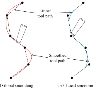
global smoothing and local smoothing [10], as shown

in Fig. 1.

(a) Global smoothing （b）Local smoothing Linear

tool path

Smoothed tool path

Fig. 1. Linear toolpath smoothing

Local Corner Smoothing Transition Algorithm Based

on Double Cubic NURBS for Five-axis Linear Tool Path

Zhang, L. – Zhang, K. – Yan, Y.

Liqiang Zhang1,* _{– Kai Zhang}1 _{– Yecui Yan}2

1 _{Shanghai University of Engineering Science, College of Mechanical Engineering, China} 2 _{Shanghai University of Engineering Science, Automotive Engineering College, China}

A five-axis tool path is often composed of a linear path that has a tangential discontinuity so that the tangential velocity will be abrupt or be equal to zero at the corner of the adjacent segments. Therefore, it greatly affects the machining efficiency and quality. Thus, a corner smoothing transition algorithm based on double cubic NURBS, which is curvature-continuous and satisfies the given accuracy constraint, is proposed to smooth the local corner at the adjacent five-axis linear path. On the basis of the smoothing transition model, the parametric synchronization between the smoothed double NURBS trajectories and the remaining two linear segments are respectively constructed to realize the smoothing variation along the tool tip translational trajectory and tool axis rotational trajectory. The simulation and examples show that the proposed transition algorithm can satisfy the error constraints, reduce the feedrate fluctuation, and improve the machining quality.

Keywords: five-axis machining, corner transition, double NURBS curves, tool path

Highlights

• A corner smoothing transition algorithm based on double cubic NURBS is proposed to smooth the five-axis linear tool path. • The proposed algorithm is curvature-continuous and satisfies the given accuracy constraint.

• The approximation error has an analytical relationship with the transition length of the smoothed curve.

Global smoothing means that the discrete tool points are approximated or interpolated by using one parametric curve to generate the smooth toolpath with G1 _{and above continuity. Langeron et al. [11] proposed}

a new method to generate the five-axis tool path by double NURBS, which described the trajectories of the tool tip points and the tool axis points, respectively.

Li et al. [12] extended the three-axis NURBS codes

format to five-axis machining by the double NURBS interpolation method to smooth the linear five-axis

tool path. Bi et al. [13] presented compact

dual-NURBS tool paths with isometric distance algorithm to smooth the linear five-axis tool paths and used the quaternion to realize the spatial motion of the tool. All the above methods are performed in a work coordinate system (WCS), and some smoothing algorithm are also realized in a machine coordinate system (MCS) [14] and [15]. Li et al. [16] proposed a linear five-axis toolpath smoothing algorithm based on double NURBS in MCS.

The local smoothing means that a smooth curve satisfying the predefined error constraint was inserted at the corner of two adjacent linear segments to realize the smoothness and continuity of the linear tool path. In recent years, more and more methods have been

developed for three-axis corner smoothing [17] to

[19]. However, because it is difficult to realize the

smoothing of the tool orientation for five-axis tool paths, there have been only a few studies and further effort should be made on this subject. Buedaert et al.

[5] presented a five-axis corner rounding method to

smooth the tool path satisfying the acceleration and jerk limit. Two B-Spline curves were inserted at the corner of the tool path to smooth the tool tip trajectory and the tool orientation, respectively. Shi et al. [20] proposed a smoothing method to round the corners of the five-axis tool paths with a pair of quintic PH curves, in which one curve rounded the corner of the tool-tip trajectory and the other curve rounded the corner of the trajectory of the tool axis. Tulsyan

et al. [10] proposed a new approach to achieving the

smoothing corner by inserting quintic and septic splines for the tool tip points and tool orientations at the adjacent linear five-axis tool path, respectively.

However, the overcuts on the parts caused by the tool orientation adjustment are not strictly restricted. Thus, it remains a challenge for a five-axis NC system to maintain the requirements of machining accuracy and smoothness of the tool motion trajectory simultaneously.

In this paper, a pair of double cubic NURBS curves satisfying the predefined fitting accuracy are used to fair the corners of the adjacent five-axis linear

segments and generate the smooth toolpath with G2

continuity in WCS. The rest of this paper is organized as follows: Section 1 proposes the five-axis corner smoothing transition algorithm based on double cubic NURBS curves in WCS. Section 2 performs the synchronization of the smoothed five-axis paths. In Section 3, computational example and experiment are adopted to evaluate the validity and effectiveness of the proposed algorithm. Finally, Section 4 is the conclusion of this paper.

1 CORNER SMOOTHING TRANSITION

1.1 Local Corner Smoothing by Double Cubic NURBS Curves with G2 Continuity

The discrete tool location data in WCS, which can be acquired from the CAM module in five-axis NC machining, consists of a series of tool tip points {Ai = (xai, yai, zai), i = 1, ..., m} and a series of tool

axis vectors {Oi = (oxi, oyi, ozi)}. Therefore, the

five-axis linear tool path in WCS can be described by two linear trajectories. One represents the translational linear trajectory which is defined by a sequence of tool tip points Ai and another represents the rotational

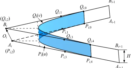
linear trajectory defined by a sequence of tool axis points (which are the second points on the tool axis) {Bi = (xbi, ybi, zbi)}, as shown in Fig. 2. The tool axis

vector Oi can be computed by the pair of tool tip

point and tool axis point (Ai, Bi). Thus, the tool tip

point, tool axis point, and tool axis vector satisfy the following relations:

Bi = Ai + H • Oi (1)

O B A

B A

i i i

i i

= −

− , (2)

where H is the distance between the tool tip point and tool axis point.

Bi-1

Ai-1

Ai+1 Bi+1 Ai

(Pi,2)

(Qi,2) Bi

Pi,3

Pi,4 Pi,0 Pi,1

Qi,0 Qi,1

Qi,3 _Q

i,4

Pi(u)

Qi(v)

Oi

H

Fig. 2. Five-axis linear tool path and corner transition curves

The term “curvature-continuous” (also called

the same curvature centre at the junction. The path

with G2 _{continuity can guarantee the continuities}

of tangency and curvature so that the fluctuation in feed, acceleration and jerk can be improved greatly. Meanwhile, the minimum degree of the NURBS curve

satisfying the G2 _{continuity is cubic. Thus, double}

cubic NURBS curves are utilized to fair the corner of the adjacent five-axis linear segments and generate

the smooth toolpath with G2 _{continuity. The smooth}

transition cubic NURBS pair, which are constrained with five control points, are respectively given as [21]:

P u

N u w P

N u w u

Q v

N i

j i j i j j

j i j

j i j

( )

( )

( )

[ ]

( )

∑

∑

4 0 1

,, , , , , , , , 3 0 4 3 0

4 0 1

v w Q

N v w v

i j i j j

j i j

j

( )

( )

[ ]

∑

∑

where Nj,3(u) are the 3rd degree B-spline basis functions

defined on the knot vector U = {0, 0, 0, 0, 0.5, 1, 1, 1, 1} and can be computed as:

N u u u

u u N u

u u

u u N u

N u

j j

j j j

j

j j j

j , , , , 3 3 2 4 4 1 1 2 0

( )

( )

( )

( )

== ≤ <         + 1 0 1 , , . if else

u_j u u_j (4)

1.2 Corner Smoothing of the Linear Trajectory of Tool Tip Points

Corner smoothing in three-axis linear segments can be regarded as the foundation of the corner smoothing in the five-axis tool path. One cubic NURBS curve is utilized to fair the corner of the translational path, and another cubic NURBS curve is used to smooth the corner of the rotational path. Thus, by inserting the double cubic NURBS curves to fair the translational and rotational paths, the corner of the five-axis linear tool path can be smoothed. Therefore, in this section, take the translational trajectory of the tool tip points as an example, the NURBS corner smoothing transition model satisfying the error constraint and G2 _continuity

will be constructed.

1.2.1 Construction of the Corner Smoothing Transition Model

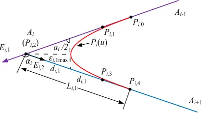
As shown in Fig. 3, the corner is formed by two adjacent segments of the translation trajectory Ai – 1Ai

and AiAi + 1. The unit vectors of the two adjacent

segments are Ei,1 and Ei + 1,1, respectively, and the

angle of the two unit vectors is α_i∈

[ ]

Ai-1

Ai+1

Ai

(Pi,2)

Pi,3

Pi,4

Pi,0

Pi,1

Pi(u) di,1

di,1

Ei,1

Ei,2

αi εi,1max

ai /2

Li,1

Fig. 3. The corner smoothing model with NURBS transition

Then the corner is rounded by a cubic NURBS

curve satisfying the error constraint and G2

continuity. Pi,0 , Pi,1 , Pi,2 , Pi,3 and Pi,4 are five control

points of the NURBS curve, and the weights are wi,0 = wi,4 , wi,1 = wi,3 and wi,2 , and the knot vector is

U = {0, 0, 0, 0, 0.5, 1, 1, 1, 1}. Meanwhile, point Pi,2

coincides with point Ai so that it is convenient to fix

the NURBS curve. In addition, the points Pi,0 , Pi,1

and Pi,3 , Pi,4 symmetrically located in linear segments

Ai–1Ai and AiAi + 1 , and satisfy the following relations:

Li,1 = | Pi,0Ai | = | AiPi,4 | , (5)

2di,1 = | Pi,1Ai | = | AiPi,3 | , (6)

where Li,1 presents the transition length of the

NURBS curve. According to [5], the relationship

between Li,1 and di,1 satisfy that

Li,1 / 2di,1 = | Pi,0Ai | / | Pi,1Ai | ∈ [1,4, 1.75]. Sets the

ratio Li,1 / 2di,1 = 1.5, then Eqs. (5) and (6) can be

reformulated as:

Li,1 = 1.5 | Pi,1Ai | = 1.5 | AiPi,3 | = 3di,1 , (7)

| Pi,1Ai | = | AiPi,3 | = 2Li,1/3 . (8)

when the tool tip points and the transition lengths are acquired, the five control points of the cubic NURBS curve can be located as:

P A L E

P A L E

P A

P A L E

i i i i

i i i i

i i

i i i i

, , ,

, , ,

,

, ,

0 1 1

1 1 1

2 3 1 2 3 2 3 = − = − =

= + ₊11 1

4 1 1 1

,

, , ,

,

Pi =A L Ei+ i i

where the transition length Li,1 must be limited by

the predefined approximation error ε, and it can be

obtained using the analytical relationship between the transition length and the approximation error shown in the next section.

1.2.2 Estimation Error of the Smoothed Curve

As shown in Fig. 3, the inconsistency of the machining path between the newly inserted transition curve and the original linear segments will cause the approximation error. Therefore, the inserted NURBS path must satisfy the constraint of the approximation error.

Because the curve Pi (u) is symmetrical with the

angular bisector of the angle ∠Ai–1 AiAi+1, the

maximal error between the transition curve and two linear segments is the distance between the midpoint of the curve Pi (u) at u = 0.5 and the point Ai , that is

|Pi (0.5) Ai |. Suppose that the approximation error, the

maximal approximation error, and the predefined approximation error are εi,1 , εi,1max and ε, respectively.

If εi,1max ≤ ε, then the approximation error between the

transition curve and the adjacent segments can be limited.

The approximation error of the transition NURBS curve must satisfy the following condition:

ε_i ε_i i i αi ε

i i

w L

w w

,1≤ ,1max=

(

)

(

)

. (10)

1.2.3 Analytical Relationship between the Transition Length and the Approximation Error

According to Eq. (10), the transition length Li,1 must

satisfy the restraint of the predefined approximation error ε, so the transition length Li,1 can be expressed

as:

L w w

w

w w

w

i i i i

i i i i i ,1 ,1max =

(

)

(

)

(

)

sin / s

ε α

ε

iin

(

)

when εi,1max = ε, the transition length Li,1 has the

maximum value, and it can be written as:

L w w

w

i i i

i i ,1= +

(

)

(

)

, sin /

.

ε

α (12)

Meanwhile, the sum of the transition lengths at the adjacent segments must not exceed the length of linear segment they lie in, that means:

L L A A

Li_i L_i i A Ai_{i i}i

− − + + + ≤ + ≤    

1 1 1 1

1 1 1 1

, ,

, ,

. (13)

It can be concluded that Li,1 satisfy the following

constraint:

L_i,1≤min

(

)

L A A A A w w

w

i i i i i i i i

i i

,

, , , max

,

min . , . ,

sin /

1 1 1

1 2 1

1

0 5 0 5 3

2

≤ − +

(

)

ε α 22

(

)

 

 _.(15)

Ai+1 Bi+1 Ai

(Pi,2)

(Qi,2)

Bi

Pi,3 _P i,4

Pi,0 Pi,1

Qi,0 Qi,1

Qi,3

Pi(u)

Qi(v)

di,1 Ei,1

Ei+1,1

αi

Ei+1,2 Ei,2

βi

Qi,4

Pi+1,0

Qi+1,0

Pi+1,4 Qi+1,4

εi,1max

εi,2max

Li,1 Li,2

di,2

Li+1,1 Li+1,2

Fig. 4. Five-axis corner transition model based on double cubic NURBS with G2 _continuity

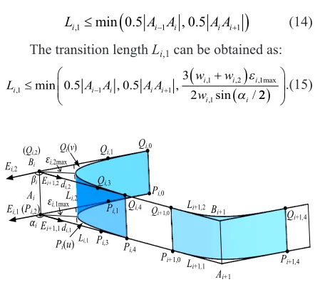
1.3 Generation of Five-Axis Corner Smoothing Model with G2 _Continuity

Similarly to the generation of the corner smoothing transition model of the translation paths, the corner smoothing transition model of the tool axis points can also be constructed. Thus, by using a series of double

cubic NURBS curves Pi(u) and Qi(v), the corners in

five-axis linear paths can be smoothed with G2

continuity, as shown in Fig. 4. The NURBS curve Pi(u) is used to smooth the corner ∠Ai–1 AiAi+1 , and

the maximal tool tip approximation error between the smoothed curve and the original linear segments is εi,1max. The NURBS curve Qi(v) is utilized to fair the

corner ∠Bi–1 BiBi+1 , and the maximum tool axis

approximation error is εi,2max. If both the maximal

approximation errors εi,1max and εi,2max are constrained

under the predefined approximation error ε as Eq.

(16), then the transition lengths can be obtained.

max(εi,1max, εi,2max) ≤ ε . (16)

Next, it is necessary to determine the maximal approximation errors εi,1max and εi,2max. In this paper,

the distance between the tool tip point and the reference tool axis point is constant with H. Taking the original tool location (Pi,0, Qi,0) as an example, the

distance between points Pi,0 and Qi,0 must satisfy the

following equation:

Left of the above equation can be computed as:

Q P B L E A L E

B A L E L

i i i i i i i i

i i i i i

, , , , , ,

, ,

0 0 2 2 1 1

1 1

− =

(

)

(

)

(

)

, max , , max ,

sin / sin /

2 2

1 1 2 2

3

2 3

2 E

H O E E

i

i i i

i i i i = = ⋅ +

(

)

(

)

(

)

(

)

, max , max

sin / sin / . (18)

If Eq. (17) is tenable, the right part of Eq. (18) must only exist H, so we can conclude that:

3 2 3 2 0 1 2 ε α ε β i i i i

, max , max

sin

(

)

(

)

The above formula can be calculated as:

3 3 2 2 1 2 ε ε α β i i i i , max , max sin /

sin / .

=

(

)

(

)

Hence, according to Eqs. (16) and (19), the

approximation errors εi,1max and εi,2max can be

determined. Then the transition lengths can be computed based on Eq. (15). Moreover, taking the transition lengths into Eq. (9), all the control points of the transition NURBS curves are given. Finally, the smoothed double cubic NURBS curves for translation paths and rotation trajectories can be written based on Eq. (3).

2 SYNCHRONIZATION OF THE SMOOTHED FIVE AXIS PATHS

After inserting a sequence of double cubic NURBS curves at the adjacent segments, the smooth

five-axis tool paths with G2 _{continuity can be generated.}

However, in five-axis tool path interpolation, both the tool-tip translation and the tool axis rotation must be guaranteed with continuous and smooth variation, so it is a key point to realize synchronous movement between the translational trajectory of tool-tip points and the rotational trajectory of tool axis points.

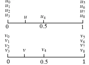
2.1 Parametric Synchronization of the Double Cubic NURBS Curves

By analysing the interpolation process along the double NURBS trajectories, the synchronous movement can be regarded as the synchronous relationship between the parameter u and v. That is, if there is parameter u ∈ [un, un+1], there must be a

parameter v with v ∈ [vn, vn+1]. In addition, the

distances between the tool tip trajectory Pi(u) and the

corresponding tool axis trajectory Qi(v) always keep a

fixed value H.

Fig. 5. Parametric synchronization between the double NURBS curves

Fig. 5 shows the parametric synchronization between the double NURBS paths. If there is parameter u ∈ [un, un+1], there must be a parameter v

with v ∈ [vn, vn+1], where n = 3, 4, and they satisfy the

following equation:

| Qi(v) – Pi(u) |= H. (20)

Supposing the parameter u of the NURBS curve

Pi(u) is known, then Eq. (20) is translated into Eq.

(21) which is solved in a given interval.

φ(v) =| Qi(v) – Pi(u) |2 – H2 = 0. (21)

Solving Eq. (21), the parameter v of the NURBS

curve Qi(v) corresponding to u can be obtained. Then

according to the relation of u and v, the tool vector corresponding to the tool-tip point can be expressed as:

O Q v P u

Q v P u

i i i

i i

= −

−

( ) ( )

( ) ( ). (22)

Thus, the tool positions in the five-axis corner paths interpolation are known. In addition, the continuous and smooth variation of the rotational trajectory is proved by using the first-order geometrical derivative of the tool vector with respect to the displacement s of the tool tip trajectory. A

detailed presentation had been proposed in [22], so

parameter u and displacement s is linked by a C3

continuous ninth-order spline, which is written as u = f(s). According to Eq. (21), the relation between u and v is simply written as v = g(u). Then there is:

dO ds dO du du ds

d Q g u P u

Q g u P u

du f s

Q g u

i i i i i i i   = ⋅ =

( )

( )

( )

( )

( )

(( ) ( )

( )

( )

( )

( )

g u P u

Q g ui P ui i f s

It can be concluded from the above equation that the rotational motion of the tool axis is continuous and smooth. Meanwhile, the tool tip point and the corresponding tool vector can be obtained.

2.2 Synchronization of the Remained Linear Tool Paths

The remaining five-axis path is the linear path between the tool positions (Pi,4, Qi,4) and (Pi+1,0, Qi+1,0) in

WCS. Therefore, the synchronization interpolation of five-axis linear paths can be achieved by constructing the parametric synchronization method between the translational trajectory and the rotational trajectory, which can be defined as:

A P

P P x

i n i

i i

i n

i i n

, ,

, , ,

, .

−

− = =

+

4

1 0 4

θ

θ (24)

Fig. 6. Synchronization of the linear tool path

As shown in Fig. 6, Pi,4 and Pi+1,0 are the control

points on the translational path, Qi,4 and Qi+1,0 are the

control points on the rotational path; both of them are obtained by using the method in Section 2.2. Setting Ai,n is any point on the translational path Pi,4Pi+1,0 ,

and it can be computed as:

Ai,n = (1 – tn) Pi,4 + tnPi+1,0 , tn∈ [0, 1]. (25)

θi is the angle between the start vector P Qi,4 i,4

and the end vector P Qi+1 0, i+1 0,

, which is expressed as:

θ_i i i i i i i

P Q P Q P Q

= ⋅ + +

arccos , , , ,

, ,

4 4 1 0 1 0

4 4

P Qi+ i+



  



  

1 0, 1 0,

, (26)

where θi,n is the angle between the start vector P Qi,4 i,4

and the vector at any position of the path Pi,4Pi+1,0 and

it can be obtained by Eqs. (24) to (26). Next, the unit vector Ori n,

at any position of the

path Pi,4Pi+1,0 can be obtained according to the

rotation formula in [23]:

O P Q P Q

O

ri n i i i n i i i

, , , , , ,

,

cos

= +

+

4 4 4 4

4

θ ⋅⋅

(

)

(

)

(

)

(27)

in which P Qi,4 i,4

is the unit vector of the tool vector

P Q_i,4 _i,4

and can be calculated as:

O Q P

Q P

i i i

i i

,

, ,

, ,

.

4

4 4

4 4

= −

− (28)

Thus, by utilizing the method in Sections 1.2.1 and 1.2.2, the tool tip points and the corresponding tool vector in five-axis interpolation are obtained, and the parametric synchronization interpolation between the remained two linear paths and the double NURBS paths are constructed to achieve continuous and smooth variation along the translational trajectory and rotational trajectory.

3 COMPUTATIONAL EXAMPLE AND EXPERIMENT VALIDATION

In this section, the proposed local corner smoothing transition algorithm based on double cubic NURBS is utilized to fair the corners for five-axis linear tool paths. Two examples are adopted to evaluate the validity and effectiveness of the proposed algorithm.

3.1 Example 1

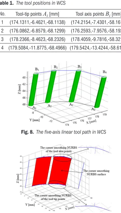
In this experiment, a flank-milling simulation for an impeller is used to generate the linear five-axis path formed by discrete tool data in WCS, as shown in Fig. 7. For the convenience of description, four tool positions are chosen to describe the proposed corner smoothing transition algorithm. Each of the tool positions consists of the tool-tip point Ai, and the tool

axis point Bi, and their coordinates are shown in Table

1.

The linear five-axis path of the four tool positions in WCS is generated by MATLAB, as shown in Fig. 8. Then, the proposed local corner smoothing transition algorithm is used to smooth the corners of linear tool paths, as shown in Fig. 9.

Fig. 7. Flank milling for an impeller part

lengths are mainly limited by the predefined approximation error and the half length of the adjacent segments. Thus, setting two groups fitting precision to smooth the corners of the linear path, as shown in Table 2, and the results show that the proposed corner-smoothing algorithm can be used to generate the double NURBS path satisfying the given precision error.

Table 1. The tool positions in WCS

No. Tool-tip points A_i [mm] Tool axis points B_i [mm] 1 (174.1311,-6.4621,-68.1138) (174.2154,-7.4301,-58.1611) 2 (176.0862,-6.8579,-68.1299) (176.2593,-7.9576,-58.1921) 3 (178.2366,-8.4623,-68.2326) (178.4059,-9.7816,-58.3215) 4 (179.5084,-11.8775,-68.4966) (179.5424,-13.4244,-58.6170)

Fig. 8. The five-axis linear tool path in WCS

Fig. 9. Five-axis corners smoothing based on double NURBS curve

Table 2. The double NURBS smoothing results under two fitting

precision restriction

No.

The approximation error for tool position (A₂, B₂)

The approximation error for tool position (A₃, B₃) Tool tip

curve [mm]

Tool axis curve

[mm] Tool tip curve [mm] curve [mm]Tool axis

1 0.0729 0.078 0.078 0.0768

2 0.0729 0.079 0.1265 0.1307

The first group result shows the maximal

approximation errors for tool positions (A2, B2)

and (A3, B3) under the constraint of the predefined

approximation error as 0.078 mm. From Table 2, both of the maximal approximation errors for tool positions (A2, B2) and (A3, B3) are 0.08 mm, which appears

at the centre points of the tool axis curve Q2(v) and

the tool tip curve P3(u). It can be concluded that the

approximation errors are influenced by the predefined approximation error. Fig. 10 shows the error distribution along the double NURBS paths, and it can be seen the approximation errors for tool positions (A2, B2) and (A3, B3) are less than the predefined error

restriction.

Fig. 10. The approximation error for tool positions (A2, B2) and

(A3, B3) under No. 1 group fitting precision

Fig. 11.The approximation error for tool positions and

under No. 2 group fitting precision

Utilizing the proposed algorithm to smooth the tool positions (A2, B2) and (A3, B3) under the

(A2, B2) and (A3, B3) are 0.079 mm and 0.1307 mm,

which appears at the center points of the tool axis curve Q2(v) and Q3(v), respectively. Fig. 11 shows the

error distribution along the double NURBS paths and all the approximation errors for tool positions (A2, B2)

and (A3, B3) do not exceed the given precision.

3.2 Example 2

As shown in Fig. 12, to verify the availability of the proposed corner smoothing and synchronization transition algorithm, the flank milling of the impeller on the five-axis machine tool with dual-table is performed by comparing the proposed algorithm and

the direct G1 _{machining method, which do not use}

corner smoothing and still maintains the linear paths. It can be seen from Fig. 13 that the results show the proposed algorithm can smooth the linear tool path of blades to satisfy the given fitting accuracy and

generate the double NURBS paths with G2 _continuity.

Fig. 12. The flank milling of an impeller

It can be seen from Fig. 13a that tool marks

obviously appear on the blades by using the G1

machining method. While the machined surfaces of the impeller using the proposed algorithm in Fig. 13b are smoother and possess better finished quality.

Both the proposed corner-smoothing algorithm

and the direct G1 _{method are implemented by setting}

the velocity as 1800 mm/min, the acceleration as 1000 mm/s2_{, the jerk as 5000 mm/s}3_{, and the interpolation}

period as 2 ms. The results of the velocity and acceleration curves are shown in Figs. 14 and 15, respectively. From the results, it can be seen that the proposed algorithm possesses higher velocity with

less fluctuation. Compared with the direct G1 _block

methods, the proposed algorithm only takes 12.074 s to machine one path of the impeller, while the direct

G1 _{method spends 14.780 s, so the machining time of}

the proposed algorithm is reduced by about 18.3%. It can be concluded that the proposed algorithm can possess a higher machining efficiency, and it can be

advantageous to improve the machining accuracy and surface quality.

a)

Tool marks

b)

Smoother surface

Fig. 13. Comparison of the impellers machining quality using two methods; a) the impeller machining quality in direct G1 _block

machining method; and b) the impeller machining quality in proposed algorithm

a)

b)

Fig. 14. Comparison of the velocity on flank milling of a blade; a) the velocity in proposed algorithm and b) the velocity in direct G1

a)

b)

Fig. 15. Comparison of the acceleration on flank milling of a blade; a) the acceleration in direct G1 _{block machining method,}

b) the acceleration in proposed algorithm

a)

b)

Fig. 16. Comparison of the error distribution on flank milling of a blade; a) the impeller machining quality in direct G1 block

machining method, and b) the impeller machining quality in proposed algorithm

To verify the availability and precision of the proposed algorithm, the machining errors on the flank milling of a blade are obtained by calculating the deviation of the machined surface. Both of the error results are achieved by setting the predefined error as 0.04 mm. Then, by using the Coordinate Measuring Machining (CMM), 70×7 points can be acquired from the machined blade to compare with the corresponding points of the surface. The error distributions of the machined surface for the two methods are shown in Fig. 16. It can be seen from Fig. 16b that the machining errors, by using the proposed methods, satisfy the predefined error 0.04 mm and most of the machining errors are less than 0.015 mm. However, most of the machining errors exceed the predefined error greatly

in the conventional G1 _{method. Thus, the comparison}

results show that the proposed corner smoothing algorithm possesses higher precision and can improve the machining surface quality significantly.

4 CONCLUSIONS

In this paper, a pair of double cubic NURBS curves satisfying the predefined fitting accuracy are utilized to fair the corners of the adjacent five-axis linear

segments and generate the smooth toolpath with G2

continuity in WCS.

The proposed algorithm has three advantages: (1) The smoothed cubic NURBS pair are constrained with five control points and can smooth the translation trajectory of the tool tip points and the tool axis points

with G2 _{continuity, respectively. Then, velocity and}

acceleration can be improved due to continuities of the tangential direction and curvature. (2) The approximation error has an analytical relationship with the transition length of the smoothed curve. It is easy to construct the analytical double NURBS curves satisfying the pre-defined error limit. (3) The synchronization method can guarantee the continuity in tool orientation variation.

5 ACKNOWLEDGEMENTS

This research is sponsored by the National Natural Science Foundation of China (No. 51305254) and the Capacity Building Project for Local Universities of the Shanghai Science and Technology Committee (No. 14110501200).

6 REFERENCES

limit. International Journal of Advanced Manufacturing Technology, vol. 48, no. 1, p. 227-241, DOI:10.1007/s00170-009-2261-y.

[2] Lasemi, A., Xue, D.Y., Gu, P.H. (2010). Recent development in CNC machining of freeform surfaces: A state-of-the-art review. Computer-Aided Design, vol. 42, no. 7, p. 641-654,

DOI:10.1016/j.cad.2010.04.002.

[3] Sencer, B. Ishizaki, K., Shamoto, E. (2015). A curvature optimal sharp corner smoothing algorithm for high-speed feed motion generation of NC systems along linear tool paths. International Journal of Advanced Manufacturing Technology, vol. 76, no. 9, p. 1977-1992, DOI:10.1007/s00170-014-6386-2.

[4] Erkorkmaz, K., Altintas, Y. (2005). Quintic spline interpolation with minimal feed fluctuation. Journal of Manufacturing Science and Engineering, vol. 127, no. 2, p. 339-349,

DOI:10.1115/1.1830493.

[5] Beudaert, X., Lavernhe, S., Tournier, C. (2013). 5-axis local corner rounding of linear tool path discontinuities. International Journal of Machine Tools and Manufacture, vol. 73, p. 9-16, DOI:10.1016/j.ijmachtools.2013.05.008.

[6] Heng, M., Erkorkmaz, K. (2010). Design of a NURBS interpolator with minimal feed fluctuation and continuous feed modulation capability. International Journal of Machine Tools and Manufacture, vol. 50, no. 3, p. 281-293, DOI:10.1016/j. ijmachtools.2009.11.005.

[7] Yau, H.T., Wang, J.B. (2007). Fast Bezier interpolator with real-time lookahead function for high-accuracy machining. International Journal of Machine Tools and Manufacture, vol. 47, no. 10, p. 1518-1529, DOI:10.1016/j. ijmachtools.2006.11.010.

[8] De Santiago-Perez, J.J., Osornio-Rios, R.A., Romero-Troncoso, R.J., Morales-Velazquez, L. (2013). FPGA-based hardware CNC interpolator of Bezier, splines, B-splines and NURBS curves for industrial applications. Computers & Industrial Engineering, vol. 66, no. 4, p. 925-932, DOI:10.1016/j.cie.2013.08.024.

[9] Chen, Z.-Z.C., Khan M.A. (2014). A new approach to generating arc length parameterized NURBS tool paths for efficient three-axis machining of smooth, accurate sculptured surfaces. International Journal of Advanced Manufacturing Technology, vol. 70, no. 5, p. 1355-1368, DOI:10.1007/s00170-013-5411-1.

[10] Tulsyan, S., Altintas, Y. (2015). Local toolpath smoothing for five-axis machine tools. International Journal of Machine Tools and Manufacture, vol. 96, p. 15-26, DOI:10.1016/j. ijmachtools.2015.04.014.

[11] Langeron, J.M., Duc, E., Lartigue, C., Bourdet, P. (2004). A new format for 5-axis tool path computation, using Bspline curves. Computer-Aided Design, vol. 36, no. 12, p. 1219-1229,

DOI:10.1016/j.cad.2003.12.002.

[12] Li, Y.Y., Wang, Y.H., Feng, J.C., Yang, J.G. (2008). The research of dual NURBS curves interpolation algorithm for high-speed five-Axis machining. Intelligent Robotics and Applications, Lecture Notes in Computer Science, vol. 5315, p. 983-992,

DOI:10.1007/978-3-540-88518-4_105.

[13] Bi, Q., Wang, Y.H., Zhu, L.M., Ding, H. (2010). An algorithm to generate compact dual NURBS tool path with equal distance for 5-axis NC machining. Intelligent Robotics and Applications, Lecture Notes in Computer Science, vol. 6425, p. 553-564,

DOI:10.1007/978-3-642-16587-0_51.

[14] Ho, M.-C., Hwang, Y.-R., Hu, C.-H. (2003). Five-axis tool orientation smoothing using quaternion interpolation algorithm. International Journal of Machine Tools and Manufacture, vol. 43, no. 12, p. 1259-1267, DOI:10.1016/ S0890-6955(03)00107-X.

[15] Beudaert, X., Pechard, P.Y., Tournier, C. (2011). 5-axis tool path smoothing based on drive constraints. International Journal of Machine Tools and Manufacture, vol. 51, no. 12, p. 958-965,

DOI:10.1016/j.ijmachtools.2011.08.014.

[16] Li, W., Liu, Y.D., Yamazaki, K. Fujisima, M., Mori, M. (2008). The design of a NURBS pre-interpolator for five-axis machining. International Journal of Advanced Manufacturing Technology, vol. 36, no. 9, p. 927-935, DOI:10.1007/s00170-006-0905-8.

[17] Pateloup, V., Duc E., Ray, P. (2010). Bspline approximation of circle arc and straight line for pocket machining. Computer-Aided Design, vol. 42, no. 9, p. 817-827, DOI:10.1016/j. cad.2010.05.003.

[18] Zhao, H., Zhu, L.M., Ding, H. (2013). A real-time look-ahead interpolation methodology with curvature-continuous B-spline transition scheme for CNC machining of short line segments. International Journal of Machine Tools and Manufacture, vol. 65, p. 88-98, DOI:10.1016/j.ijmachtools.2012.10.005.

[19] Zhang, L.B., You, Y.P., He, J., Yang, X.F. (2011). The transition algorithm based on parametric spline curve for high-speed machining of continuous short line segments. International Journal of Advanced Manufacturing Technology, vol. 52, no. 1, p. 245-254, DOI:10.1007/s00170-010-2718-z.

[20] Shi, J., Bi, Q.Z., Zhu, L.M., Wang, Y.H. (2015). Corner rounding of linear five-axis tool path by dual PH curves blending. International Journal of Machine Tools and Manufacture, vol. 88, p. 223-236, DOI:10.1016/j.ijmachtools.2014.09.007.

[21] Piegl, L., Tiller, W. (1997). The NURBS Book, Springer-Verlag, Berlin, Heigelberg, DOI:10.1007/978-3-642-59223-2.

[22] Yuen, A., Zhang, K., Altintas, Y. (2013). Smooth trajectory generation for five-axis machine tools. International Journal of Machine Tools and Manufacture, vol. 71, p. 11-19,

DOI:10.1016/j.ijmachtools.2013.04.002.