Volume 20 - Article 29 | Pages 721–730

Demographic Researcha free, expedited, online journal of peer-reviewed research and commentary

in the population sciences published by the Max Planck Institute for Demographic Research Konrad-Zuse Str. 1, D-18057 Rostock·GERMANY www.demographic-research.org

DEMOGRAPHIC RESEARCH

VOLUME 20, ARTICLE 29, PAGES 721-730

PUBLISHED 18 JUNE 2009

http://www.demographic-research.org/Volumes/Vol20/29/ DOI: 10.4054/DemRes.2009.20.29

Formal Relationships 4

The age separating early deaths

from late deaths

Zhen Zhang

James W. Vaupel

This article is part of the Special Collection “Formal Relationships”. Guest Editors are Joshua R. Goldstein and James W. Vaupel.

c

°2009 Zhen Zhang & James W. Vaupel.

1 Relationship 721

2 Proof 722

3 Numerical findings 723

4 History and related results 725

5 Applications 726

References 727

Formal Relationships 4

The age separating early deaths from late deaths

Zhen Zhang1,3

James W. Vaupel2,3

Abstract

Averting deaths may either increase or reduce life disparity, as measured bye†_{. The sign} of the effect depends on the age at which the deaths are averted. We show that there may, depending on the entropy of the life table, be an age such that averting deaths before that age reduces disparity, but averting deaths after that age increases disparity. We say that this age separates “early” from “late” deaths (in terms of their effect on disparity) and investigate the factors determining this threshold age. If life table entropy is less than one, a unique threshold age separating early and late deaths always exists. If life table entropy is greater than one, averting deaths at any age increases disparity. If entropy equals one, averting deaths at age zero has no effect, but averting a death at any age after zero increases disparity.

1. Relationship

We measure life disparity by life expectancy lost due to death,e† ₌ R∞

0 e(a)d(a)da,

wheree(a) = ¡R_a∞`(x)dx¢/`(a) is remaining life expectancy at agea and d(a) = `(a) µ(a)is the life table distribution of deaths. Note that`(a) = exp(−R₀aµ(x)dx), with`(0) = 1, gives the probability of survival to agea, that µ(a)denotes the age-specific hazard of death, and thatH(a) =R₀aµ(x)dxis the cumulative hazard function withH(0) = 0.

Consider a perturbation that alters the cumulative hazard function by a step function with a single negative step of sizes. Lete†

sbe the corresponding value of life disparity with the perturbation. To study the impact one† _{of a concentrated decrease in mortality} at agea, it is useful to consider the function

(1) k(a) = 1

`(a) de† s ds ¯ ¯ ¯ ¯ s=0

= e†(a) +e(a)¡H(a)−1¢,

1_{Max Planck Institute for Demographic Research. E-mail: [email protected]} 2_{Max Planck Institute for Demographic Research. E-mail: [email protected]}

wheree†_{(a) =}¡R∞

a e(x)d(x)dx

¢

/`(a)is life expectancy lost due to death among people surviving to agea. Mortality reductions at ages withk <0decrease life disparity, while those at ages withk >0increase life disparity.

We prove below that ife†_{/e(0) < 1, then there exists an agea}† _{greater than zero} such thatk > 0 for a greater than a† _{andk < 0 for values of a less than a}†_{. We} also prove that ife†_{/e(0) = 1, then averting a death at age zero does not change life} disparity, but averting a death at any higher age increases disparity. Finally we prove that ife†_{/e(0)>1, then averting a death at any age increases life disparity. In the proof we} make use of the fact thatk(0) =e†_{−e(0). Note that the “entropy of the life table” equals}

e†_{/e(0)(Keyfitz 1977; Mitra 1978; Goldman and Lord 1986; Vaupel 1986), which differs} from the standard statistical definition by a term equal tolne(0). If life table entropy is less than one, thenk(0)<0; if entropy is one, thenk(0) = 0; and if entropy is greater than one, thenk(0)>0.

2. Proof

We consider three cases.

Case 1:k(0)<0 (entropy<1)

Because life spans are finite, `(a) approaches zero and H(a) approaches infinity. Therefore at an old enough agex, H(x) > 1 andk(x) > 0. Since k(0) < 0 and

k(a)is continuous, the intermediate value theorem implies that there exists at least one point, sayz, in[0,∞]such thatk(z) = 0. We prove that at any such root the derivative ofkis positive. This implies the root is unique, as shown in the Appendix.

The derivative of (1) is given by

dk(a) da =

de†_(a)

da + ³

H(a)−1 ´_de(a)

da +e(a)

d¡H(a)−1¢ da

=−µ(a)e(a) +µ(a)e†_{(a) +}¡_H(a)−1)¢¡_{µ(a)e(a)−1}¢_+e(a)µ(a) (2)

=µ(a)e†_{(a) +}¡_H(a)−1)¢¡_{µ(a)e(a)−1}¢_.

Whenk(a) = 0it follows from (1) thatH(a)−1 = −e†_{/e(a). Substituting this} into (2) yields

dk(a) da ¯ ¯ ¯ ¯

a=z

=µ(a)e†_(a)−e†(a)

e(a) ¡

µ(a)e(a)−1¢=e

†_(a)

e(a) >0.

Case 2:k(0) = 0 (entropy= 1)

In this case,z= 0. We need to show that this is the only value ofz, i.e., the only age whenk= 0. It follows from (2) that ifk(0) = 0then

dk(a) da

¯ ¯ ¯ ¯

a=0 = 1.

Hence k becomes positive as age increases from zero. If there were an age above zero whenk(z) = 0, then the derivative ofkat this age would have to be zero or neg-ative. But as shown in (3), the derivative has to be positive at any age whenk(z) = 0. This contradiction implies that the value ofa† _{equal to zero is unique in the case when}

k(0) = 0.

Case 3:k(0)>0 (entropy>1)

As noted above in Case 2, if there were an age whenk(a) = 0then the derivative of

kat this age would have to be zero or negative. But as shown in (3), the derivative has to be positive at any age whenk(a) = 0. This contradiction implies that there is no age that separates early from late deaths whenk(0)> 0: averting a death at any age would increase life disparity.

Q.E.D.

3. Numerical findings

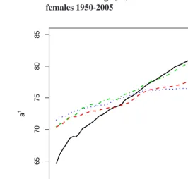
In Case 1, when entropy is less than one, to calculatea† _{it is necessary to find the age} at which e†_{(a) = e(a)}¡_1−H(a)¢_{. Using interpolation routines widely available in} statistical software,a† _{can be readily obtained, as illustrated in Figure 1. Changes ina}† over time are shown in Figure 2. The value ofa†_{in Japan increased from 65 in 1950 to} 84 in 2005. Note that a decline in mortality at age 75 before 1972 increased life disparity while such a decline after 1972 decreased life disparity.

(Coale, Demeny, and Vaughan 1983). For the Chinese womene(0) = 21.00,e† _{= 21.73,} and entropy= 1.03. For the Chinese malese(0) = 17.43,e† _{= 22.17, and entropy=}

1.27. These cases may be artifacts of bad data.

It would be interesting to determine the conditions such that the life table entropy is greater than, equal to, or less than one. Although life table entropy may rarely exceed one for human populations, this may be common for some non-human species or for some kind of machines or equipment.

Figure 1: A graphical depiction of the calculation of the threshold age (a†_),

for US females, 2005

0 20 40 60 80 100

0

20

40

60

80

Age

e

† (x)

and e(x)(1−H(x)) in Y

ears

a† e†(x)

e(x)(1−H(x))

Figure 2: The threshold age (a†_{) over time in four countries,}

females 1950-2005

1950 1960 1970 1980 1990 2000

60

65

70

75

80

85

Year

a

†

Japan USA Denmark France

4. History and related results

Based on the notion of life table entropy (Keyfitz 1977), Mitra (1978), Goldman and Lord (1986) and Vaupel (1986) independently derived the mathematical expression fore†_and showed that life table entropy equalse†_{/e(0). Vaupel and Canudas-Romo (2003) later} showed that the derivative of life expectancy over time is given by the product ofe†_and the rate of progress in reducing age-specific death rates.

Vaupel (1986) found that if the force of mortality follows a Gompertz curve,

µ(a) = µ(0)eba_{, thene}† _{≈ 1/b. The parameter b has traditionally been interpreted} as the rate of aging, but this result indicates that an alternative interpretation ofbis that it is an inverse function of life disparity.

proposed (Cheung et al. 2005). These include the variance of the age at death, the stan-dard deviation, the stanstan-dard deviation above age 10 (Edwards and Tuljapurkar 2005), the inter-quartile range (Wilmoth and Horiuchi 1999), the Gini coefficient (Shkolnikov, An-dreev, and Begun 2003), and the entropy of the life table (Keyfitz 1977). These measures are highly correlated with each other. In particular, the correlation ofe† _{with the other} measures is never less than 0.952, according to our calculations based on 5830 period life tables from 1840 to 2007 available from the Human Mortality Database (2009) (See table in Vaupel, Zhang, and van Raalte 2009). Hencee†_{can be viewed as a surrogate for} the other measures. Moreover, it turns out that the derivatives of some other measures (e.g., standard deviation of age at death, standard statistical entropy of age at death) with respect to the change in mortality have a similar form and all imply the existence of an age separating early and late deaths (Caswell, personal communication). We prefere† because of its desirable mathematical properties, used above and below, and because it can be readily explained and interpreted.

5. Applications

At the threshold agea†_{, the change ine}†_{resulting from mortality decline can be} decom-posed into two components

˙

e†(t) = de

†_(t)

dt = Z a†_(t)

0

k(a, t)d(a, t)ρ(a, t)da+ Z ω

a†_(t)

k(a, t)d(a, t)ρ(a, t)da,

(4)

whereρ(a, t)is the rate of progress in reducing death rates. The first term on the right side of (4) represents the compression of mortality at younger ages, and the second term the expansion of mortality at older ages. The balance of the two components determines whether the population experiences mortality compression or expansion (Zhang and Vau-pel 2008).

Analogously, the increase in life expectancy at birth e˙†_{(t) can be broken into two} parts,

˙ e(0, t) =

Z _a†_(t)

0

e(a, t)d(a, t)ρ(a, t)da+ Z _ω

a†_(t)

e(a, t)d(a, t)ρ(a, t)da,

(5)

References

Barclay, G.W., Coale, A.J., Stoto, M.A., and Trussell, T.J. (1976). A reassessment of the demography of traditional rural China. Population Index 42(4): 606–635.

doi:10.2307/2734378.

Cheung, S., Robine, J., Tu, E., and Caselli, G. (2005). Three dimensions of the survival curve: Horizontalization, verticalization, and longevity extension. Demography42(2): 243–258.doi:10.1353/dem.2005.0012.

Coale, A.J., Demeny, P.G., and Vaughan, B. (1983). Regional Model Life Tables and Stable Populations. New York: Academic Press, 2nd ed.

Edwards, R.D. and Tuljapurkar, S. (2005). Inequality in life spans and a new perspective on mortality convergence across industrialized countries.Population and Development Review31(4): 645–674. doi:10.1111/j.1728-4457.2005.00092.x.

Goldman, N. and Lord, G. (1986). A new look at entropy and the life table.Demography 23(2): 275–282. doi:10.2307/2061621.

Human Life-Table Database (2009). [electronic resource]. Max Planck Institute for De-mographic Research (Germany), University of California, Berkeley (USA), and Institut national d’études démographiques (France). Available atwww.lifetable.de(data down-loaded on January 10, 2009).

Human Mortality Database (2009). [electronic resource]. University of California, Berke-ley (USA) and Max Planck Institute for Demographic Research (Germany). Avail-able atwww.mortality.orgorwww.humanmortality.de(data downloaded on January 10, 2009).

Keyfitz, N. (1977).Applied Mathematical Demography. New York: John Wiley, 1st ed. Mitra, S. (1978). A short note on the Taeuber paradox. Demography15(4): 621–623.

doi:10.2307/2061211.

Shkolnikov, V., Andreev, E., and Begun, A.Z. (2003). Gini coefficient as a life table function: Computation from discrete data, decomposition of differences and empirical examples.Demographic Research8(11): 305–358. doi:10.4054/DemRes.2003.8.11. Vaupel, J.W. (1986). How change in age-specific mortality affects life expectancy.

Popu-lation Studies40(1): 147–157.doi:10.1080/0032472031000141896.

Vaupel, J.W., Zhang, Z., and van Raalte, A. (2009). Life expectancy and disparity. Paper presented at Population Association of America 2009 Annual Meeting, Detroit, April 30-May 2, 2009.

Wilmoth, J.R. and Horiuchi, S. (1999). Rectangularization revisited: Variability of age at death with human populations.Demography36(4): 475–495.doi:10.2307/2648085. Zhang, Z. and Vaupel, J.W. (2008). The Threshold between Compression and

Appendix

A simple lemma in calculus

Letfbe a real-valued differentiable function on[0,∞)with derivativef0_{and the property}

thatf0_{(x)>0wheneverf(x) = 0. Thenfhas at most one root.}

Proof. Suppose to the contrary that there are at least two roots off. First, we will show that between any two distinct roots off there is another root off. Pick any two roots of

f, sayaandbwitha < b. Sincef is differentiable ata,

lim

x→a,x>a

f(x)−f(a) x−a

exists and equalsf0_{(a). Sincef}0_{(a)>0, there is an²}

a >0such thatf(x)−f(a)>0, for allx∈(a, a+²a); that is,f is positive on the interval(a, a+²a). Analogously, there is an²b >0such thatf is negative on the interval(b−²b, b). Clearly,a+²a ≤b−²b. Thusa+²a/2< b−²b/2, andf(a+²a/2)>0andf(b−²b/2)<0. Note that, since

f0 _{exists,f is continuous on[0,∞). By the intermediate value theorem applied tof on}

[a+²a/2, b−²b/2],f vanishes at somec∈(a+²a/2, b−²b/2). Hencef(c) = 0, for somec∈(a, b).

Having shown that between any two distinct roots off there is another root off, we will use the above setup with a, b, ²a and ²b to derive a contradiction. Let

X = {x ∈ (a, b) : f(x) = 0} be the set of all roots off betweenaandb. Clearly,

X 6=∅ andX ⊂ [a+²a, b−²b]. SoX has a supremumswiths ∈ [a+²a, b−²b]. Nows = limn→∞xn, for somexn ∈X. Sincef is continuous ats, we havef(s) =

limn→∞f(xn) = limn→∞0 = 0. Sinces < b,f has a roott ∈(s, b), so thatt ∈X. This contradicts the fact thatsis the supremum ofX and finishes the proof. Q.E.D.