R E S E A R C H
Open Access
Entropy solution of fractional dynamic
cloud computing system associated with
finite boundary condition
Rabha W Ibrahim
*, Hamid A Jalab and Abdullah Gani
*Correspondence: [email protected] Faculty of Computer Science and Information Technology, University Malaya, Kuala Lumpur, 50603, Malaysia
Abstract
Cloud computing is relevant for the applications transported as services over the hardware and for the Internet and systems software in the datacenters that deliver those services. The major problem for this state is computing the capacity and the amplitude of the dynamic system of these services. In this effort, we process an algorithm based on fractional differential stochastic equation (fractional
Fokker-Planck equation (FFPE)) to find the fractional entropy solutions. Our tool is based on Mellin-Laplace transforms. Also, we suggest a fractional functional entropy formula by using the Tsallis entropy. Approximate outcomes are illustrated and discussed. The convergence of the method is investigated.
Keywords: fractional calculus; fractional dynamical system; fractional entropy; cloud computing
1 Introduction
Fractional calculus has many applications, not only in mathematics, but in other sci-ences, engineering, economics, and social studies. It covenants with differential and in-tegral operators involving arbitrary powers; real and complex. It is associated with many well-known names such as Abel, Caputo, Euler, Grunwald, Hadamard, Hardy, Heaviside, Jumarie, Laplace, Leibniz, Letnikov, Liouville, Riemann, Riesz, and Weyl. The central pur-pose, or, at least, one of the chief purposes in considering and studying fractional calculus, is the circumstance that fractional calculus appears to be fairly significant in the investiga-tion of some problems which arise in fractal space-time physics. We have physical schemes at three unalike stages of thought: microscopic, megascopic, and macroscopic. The frac-tional calculus approximates the classical calculus, and it includes non-commutative derivatives, which appears to be fairly reliable on using non-commutative geometry. This development leads one to generalize the information theory of fractional order. The books of Oldham and Spanier [], Srivastava and Owa [], Oustaloup [], Miller and Ross [], Samkoet al.[], Kiryakova [], Mainardi [], Podlubny [], Hilfer [], Zaslavsky [], Kilbas
et al.[], Magin [], Sabatieret al.[], Hilfer [], Mainardi [], Monjeet al.[], Klafter
et al.[], Tarasov [], Baleanuet al.[], Yang [], Jumarie [, ],etc.have enriched all areas of applied sciences. However, certain mathematical problems remain and baf-fle us. The complications and most of the recognized key mathematical problems in the
field have been determined up to a point. There were practically no applied formulations of requirements in different areas. The developments in these areas continue [–]. The central substantial advantage of fabricating a procedure of fractional differential equations (ordinary and partial) in scientific modeling is their nonlocal property. It is recognized that the normal derivative is a local, linear operator, while the fractional derivative is nonlocal and non-linear. As a result the subsequent formulation of a system is predisposed by not only its current formal feature, but consistently by all of its preceding ones.
The theory of entropy was introduced in the area of thermodynamics in the th cen-tury and was utilized by Shannon to improve the information theory. Entropy is a conven-tional statistic computing concept, showing uniformity and complexity, which achieves promising applications to a widespread variety of reasonable and noisy time series data. The development was motivated by data length restraints that are commonly challenging. Investigators stressed its employment and amplification, and its utility to differentiate as-sociated stochastic processes and models. They deliberated its impact and are stimulated to apply it in a statistically usable manner, such as marginal probability distributions and other methods. The major outcome is that the density of information so convoluted is formulated by the derivative of the function or its fractional derivative, depending upon whether it is differentiable or not. As regards information theory, one may compare the perspectives between the probability density and the derivative of a function. Fractional entropy appeared due to Tsallis () (see []). Many investigators published different studies to improve this concept (see [–]).
Recently, cloud computing (CC) has developed as one of the newest and most general network computing models in various areas, such as academic circles, governments, in-formation industry,etc.It is now essential for the new compeers information technology modification, and it expresses the progress of great scales, increasing focus on the rel-evance in IT studies. In an environment of CC, data is stockpiled on the cloud and ma-nipulators can attain the influential computing capability from the cloud, devoid of getting those costly substructures. A manipulator would purchase the service of CC and attain de-mand as extended as suggested to the cloud service supplier and paying the lowest price. The experimental results show that the entropy is the best method to select the service of CC (see [, ]). This study leads to the probability capacity and the amplitude of the dynamic system of these services.
In this work, we develop an algorithm based on the fractional differential stochastic equation (FFPE) to find the fractional entropy solutions. These solutions are employed to compute the capacity and the amplitude of fractional dynamic systems. Our tool is based on the Mellin-Laplace transforms. Moreover, we propose the fractional functional entropy formulated by the Tsallis concept of entropy. Numerical results are presented for illustration. The convergence of the method is investigated.
2 Processing
Our approach deals with the following concepts.
2.1 The fractional Fokker-Planck equation (FFPE)
In this effort, we consider the following fractional differential equation with diffusion co-efficients:
Dνt℘(,t) = – ∂ ∂
μ()℘(,t)+
∂ ∂
subject to the initial condition
℘(, ) :=℘()
and the boundary condition of℘(,t) is finite as→,
℘(,˜t) +℘(,t) =
+= , <t˜<t∈J= [,T],T<∞,<∞
and
℘(,t)→, ∂℘(,t)
∂ →, → ∞,
where℘() is a function of the amplitude response,℘(,t) is the density function of with respect timet∈J,Dν
t is referred to the Riemann-Liouville calculus introduced by
the formula
Dνs℘(s) = d
ds
s
(s–ς)–ν
( –ν)℘(ς)dς,
which coincides with the fractional integral operator
Iaν℘(s) =
s
a
(s–ς)ν–
(ν) ℘(ς)dς,
such thatν∈(, ). Moreover,is the capacity of the outcome of the system,℘is the probability density with respect to the capacity of the system, and the diffusion coefficients are polynomials insuch that
μ() =
n
k=
αkk, ()
σ() =β+
n
k=
βkk, ()
whereαkandβkare polynomial coefficients. Our aim is to solve equation (), by using the
fractional entropy (of Tsallis type) subject to boundary and initial conditions.
2.2 The fractional entropy
The Tsallis fractional entropy [] is formulated by
λ(℘) =
[℘()] λd–
–λ , λ= ,
or in discrete form
λ(℘) =
λ– –
m
k= ℘kλ
On this level, we require a computation of an applicable aggregate of the information cre-ated by noticing the entrance of an occurrence having probability℘∈[, ]. In this dis-cussion, we suggest the functional entropy formula
λ(℘)(,t) =
[℘(,t)] λd–
–λ , λ= .
Fractional entropy introduces in a natural way supplementary information as regards the implication of individual processes and to regulator modification. Ifλhas a large positive rate this measure is additional slight to records that arise often; nevertheless for large neg-ativeλit is slighter to the processes which arise seldom. Obviously dimension methods are attractive considering a construction in the entropy calculations. The hypothetical work was surpassing to successfully differentiate dynamical systems expecting finite, noisy data, or to confirm a deterministic background. Accordingly, in these approaches and actions, the collection of data, which is naturally significant to appreciate convergence, is impos-sibly large. By employing the fractional entropy on℘(,t), we have the fractional entropy system
Dν
tλ(℘)(,t) = – ∂ ∂
μ()λ(℘)(,t)
+
∂ ∂
σ()λ(℘)(,t)
. ()
2.3 The fractional transform
In this effort, we shall utilize the Mellin transform. This transform has a big capability in many areas such as digital data structures, probabilistic algorithms, asymptotic estima-tion of integral forms, asymptotic analysis of algorithms and communicaestima-tion theory. By applying the concept of the Mellin transform of the probability density with respect to the capacity, we have
λ(℘)(ρ– ,t) =
∞
λ(℘)(,t)ρ–d, ρ=a+ıb∈C,∈[,∞),
wherea< is the real part ofρ, whileb∈Ris the imaginary part andıis the imaginary value,√–. Obviously, the fraction transform is performed by the moment of the frac-tional complex power. In a discrete form, the converse reads as follows:
℘(,t)≈ γ
n
j=–n
℘(ρj– ,t)
ρj =
γ
n
j=
℘(ρj– ,t)
ρj ,
whereγ:=π/ b, bis the discretization level on the imaginary axis andρj:=a+ıj(π/γ).
For∈[e–γ,eγ], a calculation yields
℘(ρ– ,t) =
γ –nj=–n,j=[e–γρj+γ–eγρj–γ]/( –ρ
j)℘(ρj– ,t)
[e–γρ+γ–eγρ–γ]/( –ρ
)
. ()
In view of equation (), a comparison of two moments shows different powers with differ-ent real partsaandasuch that a=a–a, and we have the following relation:
℘
ρj()– ,t= γ
n
j=–n
℘
where
ρj(κ)=aκ+ıj(π/γ), κ= ,
and
Kj( a) =
γ[e aγ+ıjπ–e– aγ–ıjπ]
aγ+ıjπ .
Now, we multiply equation () byρ–, and integrating the outcome with respect toin the interval [,∞), we obtain the fractional system
Dν
t℘(ρ– ,t) = –
μ()℘(,t)∞ + (ρ– )
∞
ρ–μ()℘(,t)d
+
∂ ∂
σ()℘(,t)ρ–∞ –
(ρ– )
ρ–σ()℘(,t)∞
+
(ρ– )(ρ– )
∞
ρ–σ()℘(,t)d. ()
By employing the assumptions of the system and utilizing () and (), equation () can be considered as follows:
Dνt℘(ρ– ,t) = (ρ– ) n
k=
αk℘(ρ– +k,t)
+
(ρ– )(ρ– )
β℘(ρ– ,t) + n
k=
βk℘(ρ– +k,t)
. ()
Since℘(,t) is finite when→, equation () is obtained for somea, whereais the real part ofρ. Corresponding to equation (), we have the following system:
Dνtλ(℘)(ρ– ,t) = (ρ– )
n
k=
αkλ(℘)(ρ– +k,t) +
(ρ– )(ρ– )
×
βλ(℘)(ρ– ,t) +
n
k=
βkλ(℘)(ρ– +k,t)
. ()
2.4 The entropy system
The minimization method for circumventing discreteness agents has the consequence of choosing at each time step the capacity that best centers on the agents. Thus, the state of the asymptotic system completely depends on the entropy solution of the FFPE model. We aim to study and determine the global behavior (self-organization) of the systems by using the capacity.
For this purpose, we assume thatsis the agent and that the request isχs,s= , . . . ,N
(the dimension of the cloud system). By using the disposition formal relation (see []), equation () can be rewritten as follows:
Dνtλ(℘)(ρs– ,t)≈λ(℘)(ρs– ,t)
(ρs– )
γ
n
k=
αkKj( –k)
+(ρs– )(ρs– ) γ
βKj() + n
k=
βkKj( –k)
. ()
Note that equation () may have a divergent solution, but in virtue of the fractional en-tropy, all the entropy solutions of equation () are convergent and hence the probability of the capacity of the system can be computed. Equation () can be solved numerically, by applying any method or by employing fractional complex transforms as suggested in [, ].
2.5 Approximate solutions
In matrix form, equation () can be written as follows:
Dνχ(t) =ϒ χ(t), ϒ= , () subject to the initial condition
χ() =τ,
whereχ:= (χ, . . . ,χN)T,τdepends onλandρand
χ(t) =λ(℘)(ρ– ,t)
and
ϒ=(ρ– ) γ
n
k=
αkKj( –k) +
(ρ– )(ρ– ) γ
βKj() + n
k=
βkKj( –k)
.
The solution of () can be formulated by utilizing the Mittag-Leffler function
χ(t) =τEν
ϒtν, ()
where
Eν(t) :=
∞
j=
tj
It is well known thatEνshows the following asymptotic behavior (see []; Theorem ):
Eν(t)∼
νe
t/ν
, ν= . ()
Hence we have the result
χ(t)≈ τ νe
tϒ/ν
. ()
3 Results and discussion
The consequences of the adopted method to evaluate the probability of the capacity through the entropy solution is characterized by the discrete symbols. The system con-verges to the diffusion of the origin. The probability of the capacity of the integer system of (), for a fixed time, can be computed by the formal expression
℘() = θ σ()exp
μ() σ()d
,
whereθ is the normalized constant,
ν= , τ= θ
σ() and ϒ=
μ() σ()d.
The initial condition adopted above indicates the stationary states at the initial time. The justification of the suggested technique to evaluate the cost response of a system is demon-strated. Moreover, for˜t=t, the boundary condition implies that
℘() =
+
, += .
Therefore, the initial cost of the cloud system is evaluated by the above equation, which is basically determined by the boundary condition of the system (). Numerous classes of fractional boundary problems are suggested in [–].
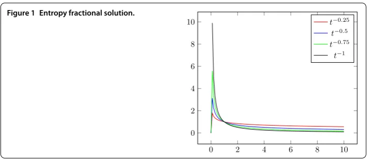
Figure 1 Entropy fractional solution.
4 Application
The job scheduling scheme is interesting and one of the essential research fields in cloud computing. It plays a similar role itself in cloud computing. The job scheduling system is accountable to choose the best appropriate resources in a cloud computing users’ jobs, by compelling various static and dynamic parameter constraints of the cloud into the de-liberation. In this section, we deal with a model that describes the job scheduling system based on the queuing property and cost function considering the users, providers, and the quality of the system (QoS). By utilizing a cloud computing environment, we may assume it as a very influential server. This server holds the user’s jobs. For each job one may have a different QoS obligation; typically, the user’s jobs have various agencies to be treated. Therefore, we can classify the jobs’ urgencies into several classes. Customarily, since the cloud computes resources, customers continuously deliberate which cloud computing re-source can encounter their job QoS supplies for computing (such as the paid time of job ruining, the calculating capacity), and how much the cost is that they must feed for the cloud computing resources.
We assume that the cloud computing system has a dynamic according to equation (). Moreover, we consider the user’s jobs in the similar group with urgency to acquiesce to the cloud agreeing to the outcomeχi(t), given in () for the useri= , . . . ,n. Each group
is evaluated by the capacity(for example, if the service has five different jobs, then the capacity obeys= , . . . , ). Suppose that the total requested groups, the service rate, and intensity of the cloud computing environment are
χ(t) =
n
i=
χi(t), f(t) = n
i=
fi(t,χ), φ(t) = n
i=
φi(t,χ), t∈J= [, ],
respectively. Then the total cost function of the cloud service is formulated by
t,χ(t),f(t),φ(t)=ωχ(t) +ωf(t) +ωφ(t) =
n
i=
ϕiχi(t), ()
whereαi,i= , . . . ,n, are the connection constants in the cloud. The problem for the cloud
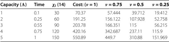
Table 1 The cost function withτ= 1,λ= 2,ρ= 2
Capacity () Time χi(14) Cost: (ν= 1) ν= 0.75 ν= 0.5 ν= 0.25
1 0.1 30 70.37 57.444 39.712 19.412 2 0.25 60 191.25 156.122 107.928 52.758 3 0.55 90 203.78 166.351 115 56.215 4 0.75 120 420.16 342.687 237.11 115.9 5 1 150 550.89 449.7 310.88 151.969
by using the fractional calculus (see Table ); here, for useri, we selectϕi∈(, ] for all
i= , . . . ,nand
ϒi=
(ρ– ) γ
n
k=
αkKi( –k) +
(ρ– )(ρ– ) γ
βKi() + n
k=
βkKi( –k)
,
corresponding to the solutionχisuch that
Ki( a) =
γ[e aγ+ıiπ–e– aγ–ıiπ]
aγ+ıiπ .
The QoS vector of the unique serviceiis defined as
Q() =ξ(ϕχ), . . . ,ξn(ϕnχn)
,
whereξiis the value of QoS parameterifor a unique service.
Table shows the initial service rate and expectant service rate for each group in the queue with changed significance. Fractional calculus is utilized to minimize the cost. The decreasing of the fractional valueν∈(, ] implies the minimization of the cost function.
4.1 Discrete cloud system
We consider the discrete cloud system of equation (), by utilizing the formula
Dνtλ(℘)( ,t) = M
k=
ω( k)λ(℘)( k,t), ()
where is the difference operator that the capacity changes in the cloud system and
λ(℘) is the fractional Tsallis entropy of orderλ= . Our aim is to find the entropy solution
of the system (). Our tool is based on the concepts of the Laplace and Mellin transforms. Sinceλ(℘) is the entropy of the distribution function℘, we may assume that
λ(℘)( ,t) :=f(t)θ( ).
Thus the system () becomes
Dνtf(t)θ( ) =
M
k=
ω( k)f(t)θ( ). ()
Since the fractional derivative is due to the time part, equation () can be read as the evolution of a fractional Brownian motion,
whereεdepends on the value of the capacity. A computation implies that the Laplace and Mellin transforms of () formally are
f(t)(ρ– ,t) =
( –ρ)∠(f(t),u)( –ρ,t), ()
where∠(f(t),u) is the Laplace transform of the functionf(t) given by
∠f(t),u=
∞
e–utf(t)dt.
Therefore, we have the following solution, in view of the Laplace transform:
f(u) = f
ε+uν, ()
wherefis a constant. Employing () in () and inverting the result to the time domain, we obtain
f(t) =
f ν
tν–F
ε/ν(, /ν) (, /ν)( –ν, )
, ()
whereF
is the well-known Fox function. In the sequel, we suppose that the value of
ω=ε= ( )
behaves as a diffusion constant. Hence by utilizing the series expansion of the Fox function (see []), the entropy solution of equation () can be described as follows:
λ(℘)( ,t) = (/ν)
∞
n=
(–)n
(nν+ )
( )tνn, f= , ()
which is a monotonic decreasing function showing the asymptotic behavior (see [])
λ(℘)( ,t)≈t–ν, t→ ∞.
5 Conclusion
Competing interests
The authors declare that they have no competing interests.
Authors’ contributions
All the authors jointly worked on deriving the results and approved the final manuscript.
Acknowledgements
The authors would like to thank the referees for giving useful suggestions for improving the work. This research is supported by Project UM.C/625/1/HIR/MOE/FCSIT/03.
Received: 21 February 2016 Accepted: 28 April 2016 References
1. Oldham, KB, Spanier, J: The Fractional Calculus (1974)
2. Srivastava, HM, Owa, S: Univalent Functions, Fractional Calculus, and Their Applications. Ellis Horwood, Chichester (1989)
3. Oustaloup, A: La commande CRONE: commande robuste d’ordre non entier. Hermes, Paris (1991) 4. Miller, KS, Ross, B: An Introduction to the Fractional Calculus and Fractional Differential Equations (1993)
5. Samko, SG, Kilbas, AA, Marichev, OI: Fractional Integrals and Derivatives: Theory and Applications. Gordon & Breach, Yverdon (1993)
6. Kiryakova, V: Generalized Fractional Calculus and Applications. Longman, New York (1994)
7. Mainardi, F: Fractional calculus. In: Carpinteri, A, Mainardi, F (eds.) Fractals and Fractional Calculus in Continuum Mechanics. CISM Courses and Lectures, vol. 378, pp. 291-348 (1997)
8. Podlubny, I: Fractional Differential Equations. Academic Press, San Diego (1999)
9. Hilfer, R (ed.): Applications of Fractional Calculus in Physics, vol. 128. World Scientific, Singapore (2000) 10. Zaslavsky, GM: Hamiltonian Chaos and Fractional Dynamics. Oxford University Press, London (2005)
11. Kilbas, AA, Srivastava, HM, Trujillo, JJ: Theory and Applications of Fractional Differential Equations. North-Holland Mathematics Studies, vol. 204. Elsevier, Amsterdam (2006)
12. Magin, RL: Fractional Calculus in Bioengineering. Begell House, Redding (2006)
13. Sabatier, J, Agrawal, OP, Machado, JAT: Advances in Fractional Calculus, vol. 4, no. 9. Springer, Dordrecht (2007) 14. Hilfer, R: Threefold introduction to fractional derivatives. In: Anomalous Transport: Foundations and Applications,
pp. 17-73 (2008)
15. Mainardi, F: Fractional Calculus and Waves in Linear Viscoelasticity: An Introduction to Mathematical Models. World Scientific, Singapore (2010)
16. Monje, CA, Chen, Y, Vinagre, BM, Xue, D, Feliu-Batlle, V: Fractional-Order Systems and Controls: Fundamentals and Applications. Springer, London (2010)
17. Klafter, J, Lim, SC, Metzler, R: Fractional Dynamics: Recent Advances. World Scientific, Singapore (2011) 18. Tarasov, VE: Fractional Dynamics: Applications of Fractional Calculus to Dynamics of Particles, Fields and Media.
Springer, Berlin (2011)
19. Baleanu, D, Diethelm, K, Scalas, E, Trujillo, JJ: Fractional Calculus: Models and Numerical Methods. Series on Complexity, Nonlinearity and Chaos, vol. 3. World Scientific, Singapore (2012)
20. Yang, X-J: Advanced Local Fractional Calculus and Its Applications. World Science, New York (2012)
21. Jumarie, G: Fractional Differential Calculus for Non-Differentiable Functions: Mechanics, Geometry, Stochastics, Information Theory. Lambert Academic Publishing, Saarbrucken (2013)
22. Jumarie, G: Maximum Entropy, Information Without Probability and Complex Fractals: Classical and Quantum Approach. Fundamental Theories of Physics, vol. 112. Springer, Dordrecht (2013)
23. Tsallis, C: Introduction to Nonextensive Statistical Mechanics: Approaching a Complex World. Springer, New York (2009)
24. Machado, JAT: Entropy analysis of integer and fractional dynamical systems. J. Appl. Nonlinear Dyn.62, 371-378 (2010)
25. Machado, JAT: Entropy analysis of fractional derivatives and their approximation. J. Appl. Nonlinear Dyn.1, 109-112 (2012)
26. Machado, JAT: Fractional order generalized information. Entropy16, 2350-2361 (2014)
27. Machado, JAT: Entropy analysis of systems exhibiting negative probabilities. Commun. Nonlinear Sci. Numer. Simul. 36, 58-64 (2016)
28. Lopes, AM, Machado, JAT: Entropy analysis of industrial accident data series. J. Comput. Nonlinear Dyn.11(3), 031006 (2016)
29. Ibrahim, RW, Jalab, HA: Existence of entropy solutions for nonsymmetric fractional systems. Entropy16, 4911-4922 (2014)
30. Ibrahim, RW, Moghaddasi, Z, Jalab, HA: Fractional differential texture descriptors based on the Machado entropy for image splicing detection. Entropy17, 4775-4785 (2015)
31. Ibrahim, RW, Jalab, HA: Existence of Ulam stability for iterative fractional differential equations based on fractional entropy. Entropy17, 3172-3181 (2015)
32. Ibrahim, RW, Jalab, HA, Gani, A: Cloud entropy management system involving a fractional power. Entropy18, 1-11 (2016)
33. Jiang, R, Liao, H, Yang, M, Li, C: A decision-making method for selecting cloud computing service based on information entropy. Int. J. Grid Distrib. Comput.8(4), 225-232 (2015)
34. Di Paola, M: Complex fractional moments and their use for the solution of the Fokker-Planck equation. In: Vienna Congress on Recent Advances in Earthquake Engineering and Structural Dynamics, 28-30 August, Vienna, Austria, pp. 28-30 (2013)
35. Ibrahim, RW: Fractional complex transforms for fractional differential equations. Adv. Differ. Equ.2012, 192 (2012) 36. Ibrahim, RW: Complex transforms for systems of fractional differential equations. Abstr. Appl. Anal.2012, Article ID
37. Gerhold, S: Asymptotics for a variant of the Mittag-Leffler function. Integral Transforms Spec. Funct.23(6), 397-403 (2012)
38. Yang, XJ, Baleanu, D, Lazarevi´c, MP, Caji´c, MS: Fractal boundary value problems for integral and differential equations with local fractional operators. Therm. Sci. (2015). doi:10.2298/TSCI130717103Y
39. Ibrahim, RW, Jalab, HA: Discrete boundary value problem based on the fractional Gâteaux derivative. Bound. Value Probl.2015, 23 (2015)
40. Ahmad, B, Agarwal, RP, Alsaedi, A: Fractional differential equations and inclusions with semiperiodic and three-point boundary conditions. Bound. Value Probl.2016, 28 (2016)
41. Srivastava, HM, Singh Chandel, RC, Vishwakarma, PK: Fractional derivatives of certain generalized hypergeometric functions of several variables. J. Math. Anal. Appl.184(3), 560-572 (1994)
42. Bas, E, Metin, F: Fractional singular Sturm-Liouville operator for Coulomb potential. Adv. Differ. Equ.2013, 300 (2013) 43. Ansari, A: Some inverse fractional Legendre transforms of gamma function form. Kodai Math. J.38(3), 658-671 (2015) 44. Khosravian-Arab, H, Dehghan, M, Eslahchi, MR: Fractional Sturm-Liouville boundary value problems in unbounded
domains: theory and applications. J. Comput. Phys.299, 526-560 (2015)
45. Sat, M, Panakhov, ES: Spectral problem for diffusion operator. Appl. Anal.93(6), 1178-1186 (2014)
46. Sat, M, Panakhov, ES: A uniqueness theorem for Bessel operator from interior spectral data. Abstr. Appl. Anal.2013, Article ID 713654 (2013)
47. Micula, S: On spline collocation and the Hilbert transform. Carpath. J. Math.31(1), 89-95 (2015)
48. Marin, M: An evolutionary equation in thermoelasticity of dipolar bodies. J. Math. Phys.40(3), 1391-1399 (1999) 49. Marsavina, L, Craciun, M: The asymptotic stress field for free edge joints under small-scale yielding conditions. An.