FREE SURFACE FLOW OVER A TRIANGULAR DEPRESSION

(1)

FREE SURFACE FLOW OVER A TRIANGULAR DEPRESSION

A. MERZOUGUI1, A. LAIADI2

Abstract. Two-dimensional steady free-surface flows over an obstacle is considered. The fluid is assumed to be inviscid, incompressible and the flow is irrotational. Both gravity and surface tension are included in the dynamic boundary conditions. Far up-stream, the flow is assumed to be uniform. Triangular obstruction is located at the channel bottom. In this paper, the fully nonlinear problem is formulated by using a boundary integral equation technique. The resulting integro-differential equations are solved iteratively by using Newton’s method. When surface tension and gravity are in-cluded, there are two additional parameters in the problem known as the Weber number and Froude number. Finally, solution diagrams for all flow regimes are presented.

Keywords: Free surface ﬂow, Potential ﬂow, Weber number, Surface tension, Froud number.

AMS Subject Classiﬁcation: 76B10, 76C05,76M25.

1. Introduction

Flow over submerged obstacles is one of the classical problems in fluid mechanics. This problem has many related physical applications ranging from the flow of water over rocks to atmospheric, and oceanic stratified flows encountering topographic obstacles, or even a moving pressure distribution over a free surface. Free surface flows over an obstacle

have been investigated for diﬀerent bottom topography by many researchers. Forbes

and Schwartz [3] used the boundary integral method to find fully nonlinear solutions of subcritical and supercritical flows over a semi-circular obstacle. Their results confirmed and extended Lamb’s solutions. In 2002, Dias and Vanden-Broeck [2] found a new solution called the ”generalized hydraulic fall”. Such solutions are characterized by downstream supercritical flow and a train of waves on the upstream side. This type of solution can be obtained by removing the radiation condition on the far upstream of the obstacle. Forbes [3] calculated numerical solutions of gravity-capillary flows over a semicircular obstruction. The fluid was subject to the combined effects of gravity and surface tension. Three different branches of solution were presented and compared between linear and fully nonlinear problems. In this work we compute accurate numerical solutions for the fully nonlinear problem. The problem is first formulated as an integral equation for the unknown shapes of the free surface. This equation is then discretized and the resulting algebraic equations are solved by Newton’s method. Later on, we found numerical solutions of

1 _{M’Sila University Department of Mathematics, Faculty of Mathematics and Informatic, Algeria}

e-mail: [email protected]

2 _{Biskra University, department of Mathematics, Algeria}

e-mail: laiadhi [email protected]

§ Submitted for GFTA’13, held in I¸sık University on October 12, 2013.

(2)

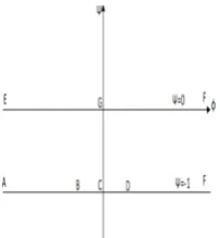
We consider the steady two-dimensional flow of an inviscid and incompressible fluid over a triangular depression. The flow is assumed to be irrotational. The fluid domain

is bounded below by a horizontal rigid wall x′ox and the triangle BCD with angle γ,

where −₂π < γ <0 and above by the free surfacesEGF. (see Figure 1). Let us introduce

Cartesian coordinates with thex−axis along the bottom and they−axis directed vertically

upwards. As x −→ ∞, the ﬂow is assumed to approach a uniform stream with constant

velocity U and constant length H. It is convenient to deﬁne dimensionless variables by

takingU as the unit velocity and H as the unit length. The dimensionless parameters in

the problem are the Froude numberF r= √U

gH and the inverse Weber numberδ =

T ρU2_H.

Here T is a surface tension, g is the gravity and ρ is a ﬂuid density. Let’s introduce

Figure 1. Sketch of the ﬂow and the coordinate

the velocity potential ϕ(x, y) and the stream function ψ(x, y), by deﬁning the complex

potential function f as :

f =ϕ(x, y) +iψ(x, y) (1)

The complex velocity ω can be written as :

ω = df

dz =u−iv (2)

where u ,v are the velocity components in thex and y directions, andz=x+iy.

We choose ϕ= 0 atG and ψ= 0 along the streamline EGF. It then follows, from the

choice of dimensionless variables, thatψ=−1 on the bottom ABCDF (Figure 2) . The

mathematical problem can be formulated in terms of the potential function ϕ satisfying

the Laplace’s equation

∆ϕ= 0 in the ﬂuid domain

The eﬀects of gravity and the surface tension are considered. Bernoulli’s equation gives

1 2

(

u∗2+v∗2)+p

∗

ρ +g

(3)

Figure 2. Flow conﬁguration in the complex potential planef =ϕ+iψ

whereu∗,v∗ are the dimensional horizontal and vertical components of velocity

respec-tively,ρis the density,p∗ is the ﬂuid pressure, g∗ is the acceleration of the gravity and B

is the dimensional Bernoulli constant. The capillary Laplace’s equation gives :

p∗−p0=

T R =K

∗_T ₍₄₎

whereK∗ = 1

R is the curvature,p

∗ _{is the ﬂuid pressure and}_p₀ _{is the atmospheric}

pres-sure. Substituting (4) into (3), used on the free surface and in terms of the dimensionless veriables, yields :

1 2

(

u2+v2)+δK+ 1

(F r)2(y−1) =

1

2 (5)

The kinematic boundary conditions are :

{

v= 0 onψ=−1 and − ∞< ϕ < ϕB and ϕD < ϕ <+∞

v=utanγ on ψ=−1 andϕB< ϕ < ϕC and ϕC < ϕ < ϕD (6)

We map the ﬂow domain from the complex potential f-plane onto the lower half of

complexζ-plane by using the conformal mapping

ζ =α+iβ=e−πf =e−πϕ(cosπψ−sinπψ) (7) as shown in ( Figure 3).

Figure 3. The ﬂow in the complexζ-plane ζ=α+iβ

Next we introduce the new complex function τ −iθ by :

(4)

∂ϕ

Substituting (9) and (10) into (5), gives the ﬁnal form of Bernoulli’s equation that is needed for the numerical calculation. This is :

1 2e

2τ₋_δeτ∂θ ∂ϕ

+ 1

(F r)2(y−1) =

1

2 on EF (11)

Using (8), the kinematic boundary conditions (6) in the ζ−plane, become :

θ = 0 − ∞< ϕ < ϕB and ϕD < ϕ <+∞and ψ=−1 (12) θ = γ ϕB< ϕ < ϕC andψ=−1

θ = −γ ϕC < ϕ < ϕD and ψ=−1

θ = unknown − ∞< ϕ <+∞ and ψ= 0

2.1. Boundary integral techniques. a diﬀerential equation was derived in terms of the

new complex variablesτ andθon the free surface. Together with the diﬀerential equation

it will define an integro-differential equation that will be solved numerically. The fluid region of the triangle problem, has an image region consisting of the upper half of the

complexζ−plane and applying Cauchy integral formula to it gives :

τ(ζ0)−iθ(ζ0) =

1

iπ

∫

Γ

τ(ζ)−iθ(ζ)

ζ−ζ0

dζ (13)

The contour Γ is a simple, where ζ0 is an image point of a point on the free surface,

i.e. ζ0 ∈EF. The path Γ consists of a large semi-circular arc of radiusR, centred at the

origin. Taking the limit of (13), asR−→ ∞,After taking the real part we obtain :

τ(α0) =−

1

π

∫ +∞ −∞

θ(α)

α−α0

dα (14)

Where τ(α0) = τ(α0,0) and θ(α) = θ(α,0) are used to simplify the notation. By

using the boundary conditions (12) the equation (14) can be written as :

τ(α0) =−

γ πlog

1 +α0

αB−α0 + γ

πlog

αD+α0

1 +α0

− 1 π ∫ +∞ 0 θ(α)

α−α0

dα (15)

This equation holds along the free surface and so using (9), with ψ= 0 gives :

α=e−πϕ (16)

Substituting (16) into (15), yields :

τ′(ϕ0) =−γ_πlog 1+e

−πϕ₀

e−πϕB+e−πϕ₀+

γ π log

e−πϕD+e−πϕ₀

1+e−πϕ₀

+∫_∞ϕ _e_−πϕθ′(ϕ₋)e_e−πϕ₋πϕ₀dϕ

(17)

for −∞< ϕ <+∞ where τ′(ϕ0) =τ

(

e−πϕ0) _and _θ′₍_ϕ_{) =}_θ(_e−πϕ)_{. The equation (11) is now rewritten in}

(5)

1 2e

2τ′ ₋_δeτ′∂θ′ ∂ϕ +

1

(F r)2(y−1) =

1

2 on EF (18)

Next we evaluate the values of y on the free surfaces by using (8) and integrating the

identity

dz df =ω

−1 ₍₁₉₎

This gives

y(α) = 1− 1

π

∫ α

0

e−τ(α0)_sin_θ₍_α

0)

α0

dα0 for 0< α <+∞ (20)

By using (16), we rewrite (20) as :

y′(ϕ) = 1 +

∫ ϕ

∞ e

−τ′(ϕ0)_sin_θ′₍_ϕ

0)dϕ0 for − ∞< ϕ <+∞ (21)

By substituting (17) and (21) into (18), an integro-diﬀerential equation is created and this is solved numerically in the following section.

3. Numerical procedure

The above system of nonlinear equations is solved numerically by using equally spaced

points in the potential functionϕ. We introduce equally spaced mesh points in the

poten-tial functionϕby :

ϕI =

[

−(N −1)

2 + (I−1)

]

∆, I = 1, ..., N,−∞< ϕ <+∞ (22)

on the upstream and downstream free surface. Here ∆>0 is the mesh sizes on upstream

and downstream free surface. The corresponding unknowns are :

θI =θ′(ϕI)

There are only N unknowns θI.We evaluate the valuesτM ofτ′(ϕ) at the midpoints

ϕM =

ϕI+1+ϕI

2 , I = 1, ..., N −1 (23)

By applying the trapezoidal rule to the integrals in (17) with summations over the points

ϕI. We evaluate yI =y′(ϕI) by applying the trapezoidal rule to (21) and by using (19).

This yields :

{

y1= 1

yI+1 =yI+ ∆e−τM sinθM

and

{

x1 =x(∞)

xI+1=xI+ ∆e−τM sinθM

I = 1, ..., N−1

Here θM =

θI+1+θI

2 . We now satisfy (18) at the midpoints (23). This yields N

nonlinear algebraic equations for theN unknowns θI, I = 1, ..., N. The derivative ∂θ

′

∂ϕ at

the mesh points (22), is approximated by a ﬁnite diﬀerence, whereby

∂θ′ ∂ϕ ≈=

θ′_I₊₁−θ′_I

(6)

are obtained with N = 250, ∆ = 0.1 and γ = −₄. We computed solutions for various

values ofN and ∆ until the numerical solutions were in agreement within graphical

accu-racy. Figure 4 shows the eﬀect of surface tension and gravity on the upstream free surface proﬁle.

-12 -10-8-6 -4 -2 0 2 4 6 8 10 0,88

0,90 0,92 0,94 0,96 0,98 1,00 1,02

(a)

-12 -10-8 -6-4 -2 0 2 4 6 8 10 0,94

0,95 0,96 0,97 0,98 0,99 1,00 1,01

Fr=0,1 Fr=0,2 Fr=0,3 Fr=0,4 Fr=0,5 Fr=0,7 Fr=0,85 Fr=1

(b)

-10 -5 0 5 10 0,970

0,975 0,980 0,985 0,990 0,995 1,000 1,005

(c)

-10 -5 0 5 10 0,93

0,94 0,95 0,96 0,97 0,98 0,99 1,00 1,01

(d)

Figure 4. (a)Free streamline shapes forF = 0 and various inverse Weber

number. (b)Free streamline shapes forδ = 0 and various Froud number Fr.

(c)Subcritical ﬂows for Fr=0.5 and δ = 0.1, 0.3 and 0.4 (d) Supercritical

(7)

References

[1] G.K Batchelor, (1967),An introduction To ﬂuid dynamics, Universit´e de Campridge.

[2] Dias, F., Vanden-Broeck, J.-M, (1989), Open channel ﬂows with submerged obstructions. J. Fluids. Mech., 206, 155–170.

[3] L. K. Forbes and L. W. Schwartz, (1982), Free-surface ﬂow over a semicircular obstruction. J. Fluid Mech., 114: 299-314.

[4] S.N.hanna, M.N.Abel-Malek et M.B.Abd-el-Malek, (1996), Super-critical free surface over trapezoidal obstacle, Journal of Computation and applied Math.66, 279-291.

[5] A.Merzougui, H.Mekias, and F.Guechi, (2007),A waveless two-dimensional ﬂow in a channel against an inclined wall with surface tension eﬀect, J.Phys, A: Math.Theor. 40.14317.