3
Multidimensional Dynamic Modeling of Milk Ultrafiltration Using
Neuro-Fuzzy Method and a Hybrid Physical Model
Y. Babazadeh1, S. M. Mousavi1∗, M. R. Akbarzadeh2
1- Department of Chemical Engineering,Ferdowsi University of Mashhad, Mashhad, Iran. 2- Department of Electrical Engineering, Ferdowsi University of Mashhad, Mashhad, Iran.
The author is also currently a visiting scholar at Berkeley Initiative on Soft Computing (BISC), University of California at Berkeley.
Abstract
Prediction of the dynamic crossflow ultrafiltration rate of a protein solution such as milk poses a complex non-linear problem as the filtration rate has a strong dependence on both the solution physicochemical conditions and the operating conditions. As a result, the development of general physics-based models has proved extremely challenging. In this study an alternative dynamic neuro-fuzzy model for milk ultrafiltration that describes the variation in dynamic permeate flux decline with temperature, transmembrane pressure (TMP), fat percentage, pH and molecular weight cut off (MWCO) has been developed with the experimental data of the pilot spiral wound membrane test rig. By increasing the temperature, TMP, and pH the permeate flux is increased, and by increasing fat concentration the permeate flux is decreased. The MWCO variation indicates a paradoxical permeate flux. Additionally, a hybrid physical model for dynamic prediction of total resistance in the milk ultrafiltration by combination of two neuro-fuzzy (ANFIS) models and a physical model (BLA model) is developed. By increasing the TMP and fat concentration, the total resistance is increased. But by increasing the pH and temperature, the total resistance is decreased. Also, MWCO variation indicates a paradoxical total resistance value.
Keywords: ultrafiltration, dynamic modeling, milk, neuro-fuzzy, hybrid model
∗ Corresponding author: E-mail: [email protected]
1- Introduction
Ultrafiltration (UF) is a membrane process that retains soluble macromolecules such as proteins and anything larger, while passing solvent, ions, and other small soluble species [1]. Ultrafiltration has now become an increasingly important industrial process for the concentration, purification, or dewatering of milk or whey. One of the main problems
4 Iranian Journal of Chemical Engineering, Vol. 5, No. 2 permeate flux and the transmission of protein
molecules, and changes the separation characteristics of the actual membrane [2]. These, in turn, lead to increased operating cost and reduced process efficiency. As a result, prediction of permeate flux and total resistance of an ultrafiltration unit are essential for process design and control. Up to now, there have been many theoretical approaches to the prediction of the rate of crossflow ultrafiltration of protein solutions [2, 3]. These are based on a wide range of phenomena such as gel polarization, boundary layer resistance, inertial migration, shear induced hydrodynamic diffusion, scour, turbulent burst, friction force, particle adhesion, pore blocking, surface renewal and particle-particle interactions. Despite the complexity of the problem, each of these approaches has indeed been shown to be valid for certain types of process feeds and under certain conditions. However, these methods also have a number of limitations as listed below:
(i) They require experimental data for hard-to-measure parameters. While this may not seem to be a practical limitation, the required equipment is usually especially sensitive instru-ments and may not be readily available.
(ii) None of the methods can describe the full flux–time (dynamic) behavior of the process; they often only predict the steady or pseudo-steady-state flux.
(iii) Each one has been shown to be valid only for certain feeds and under special conditions [3-5].
(iv) These models could not employ all parameters of the process into one formulation.
Because of these limitations, alternative modeling methods are considered for direct process modeling from historical input-output data. Artificial neural networks (ANNs) present one such paradigm that has shown a strong ability to model nonlinear
complex processes. In previous works, ANNs were used for modeling the membrane process [3-7]. However, the resulting network of weight matrices is hard to interpret.
A different data-driven approach, based on neuro-fuzzy paradigm, aims to merge traditional ANN with fuzzy logic in order to use both methods to their advantage. A neural network can approximate a function, but it is impossible to interpret the result in terms of natural language. The fusion of neural networks and fuzzy logic in neuro-fuzzy models may provide learning as well as better interpretability. Engineers find this feature useful, because the models can be interpreted and supplemented more easily by process operators.
However, fusion of neural networks and fuzzy logic does not completely solve the problem of interpretability as the overall approach generally remains one of “black box” models. Hybrid physical models aim to remedy this problem. In hybrid physical models, data driven models are combined with physical models. These models are called “grey box” models because they describe mechanisms of the process to a certain extent.
In this study, a neuro-fuzzy model and a hybrid physical model are developed for the milk ultrafiltration process where the latter consists of two neuro-fuzzy models and a boundary layer adsorption model (resistances in series model). The aim of this work is to use the proposed black box and hybrid grey-box modeling approach to study how operational and physicochemical properties affect dynamic permeate flux and the total resistance of milk ultrafiltration.
2- Theory
2-1- Fuzzy logic
Iranian Journal of Chemical Engineering, Vol. 5, No. 2 5 aspects of human knowledge and reasoning
processes without employing precise quantitative analyses. Fuzzy set theory and fuzzy logic were established in 1965 by Zadeh in order to deal with the vagueness and ambiguity associated with human thinking, reasoning, cognition, and perception [8]. After Zadeh’s work on fuzzy sets, many theories in fuzzy logic were developed, and fuzzy modeling or fuzzy identification has been applied successfully to a number of applications [9, 10]. A fuzzy model is one that expresses a complex system in the form of fuzzy implications. In the fuzzy modeling of a process, a fuzzy model is built using the physical properties of a system, observed data, as well as empirical knowledge. A typical fuzzy logic system consists of four major components: fuzzification interface, fuzzy rule base, fuzzy inference engine, and defuzzification interface [11].
The fuzzification interface (fuzzifier) converts numerical input data into suitable linguistic terms, which may be viewed as labels of the fuzzy sets. A fuzzy rule represents a fuzzy relation between two fuzzy sets. It takes a form such as “If X is A then Y is B”. Each fuzzy set is characterized by appropriate membership functions that map each element to a membership value between 0 and 1. A fuzzy rule base contains a set of fuzzy rules, where each rule may have multiple inputs and multiple outputs. Fuzzy inference can be realized by using a series of fuzzy operations. The defuzzification interface (defuzzifier) combines and converts linguistic conclusions (fuzzy membership functions) into crisp numerical outputs. Depending on the types of inference operations upon “if-then rules”, three types of fuzzy inference systems have been widely employed in various applications: Mamdani fuzzy models, Sugeno fuzzy models, and Tsukamoto fuzzy models. The differences between these three fuzzy inference systems lie in the consequents of their fuzzy rules, and thus their aggregation
and defuzzification procedures differ accordingly [12].
2-2- Neural Networks
6 Iranian Journal of Chemical Engineering, Vol. 5, No. 2
Layer 1 Layer 2 Layer 3 Layer 4 Layer 5
A1
A2
B1
B2
X1
X2
Y
adjusted to minimize the error between the network output and the actual value. The back-propagation training algorithm is an iterative gradient algorithm, designed to minimize the mean square error between the predicted output and the desired output. The flow chart of the back-propagation learning algorithm is illustrated in Fig. 1 [13, 14].
Figure 1. The algorithm of training a back
propagation network
2-3- Adaptive neuro-fuzzy inference system (ANFIS)
While fuzzy logic performs an inference mechanism under cognitive uncertainty, computational neural networks offer exciting advantages, such as learning, adaptation, fault tolerance, parallelism, and generalization. To enable a system to deal with cognitive uncertainties in a manner more like humans, neural networks have been engaged with fuzzy logic, creating a new terminology called neuro-fuzzy method [15]. Takagi and Hayashi pioneered augmentation in development of neuro-fuzzy technology in the last decade. Similarly, Jang developed ANFIS (Adaptive Neuro Fuzzy
Inference Systems) in the early 90s [16]. As the name suggests, ANFIS combines the fuzzy qualitative approach with the neural networks adaptive capabilities to achieve a desired performance. ANFIS are fuzzy models put in the framework of adaptive systems to facilitate learning and adaptation. Such systems can be trained with no need for the expert knowledge that is usually required for the design of the standard fuzzy logic. Fig. 2 shows the ANFIS architecture. A first order TSK fuzzy model is used as a means of modeling fuzzy rules into desired outputs:
Figure 2. Schematic of a neuro-fuzzy structure
If X1 = Ai and Xn= Bj then fi = piX1 + qiXn +ri
where pi , qi and ri are design parameters to
be determined during the training stage. In the presentation, a circle indicates a fixed node whereas a square indicates an adaptive node. An adaptive node means that the parameters are changed during adaptation or training. This architecture is a five-layered feed-forward neural structure, and the functionality of the nodes in these layers is summarized as follows:
Iranian Journal of Chemical Engineering, Vol. 5, No. 2 7 OL1i = µAi(X1) (1)
2. The nodes in layer 2 are fixed (not adaptive). Each node in this layer estimates the firing strength (wi) of a
rule, which is found from the multiplication of the incoming signal:
OL2i = wi = Ai(X1)µBj(Xn) (2)
3. The nodes in layer 3 are also fixed nodes. Each node in this layer estimates the ratio (wi) of the ith rule’s firing strength to sum of the firing strength of all rules, j. They perform a normalization of the firing strength from the previous layer. The output of each node in this layer is given by:
∑
= − = = i j i i i i w w w OL 13 (3)
4. All the nodes in layer 4 are adaptive nodes. The output of each node in this layer is the product of the previously found relative firing strength of the i th rule (referred to as defuzzifier or consequent parameters) and the rule (a first order polynomial for first order Sugeno model):
) (
4i w_i fi w_i piX1 qiXn ri
OL = = + + (4)
Where pi, qi and ri are design parameters
(referred to as consequent parameters since they deal with the then-part of the fuzzy rule).
5. Layer 5 has only one node, and it performs the function of a simple summer. It computes the overall output as the summation of all incoming signals from layer 4:
∑
∑
∑
= = = − i i i i i i j i i i w f w f w OL 1 5 (5)The results are then defuzzified using a weighted-average procedure. The ANFIS architecture is not unique. Some layers can be combined and still produce the same output. In this ANFIS architecture, there are two adaptive layers (layers 1 and 4). Layer 1 has modifiable parameters related to the input membership function. The parameters in this layer are called premise parameters. Layer 4 has also three modifiable parameters (pi, qi and ri) pertaining to the first order polynomial. These parameters are called consequent parameters. The task of the training or learning algorithm for this architecture is to tune all the modifiable parameters to make the ANFIS output match the training data. A training method such as back-propagation or a hybrid learning rule which combines the gradient method and the least squares is employed to find the optimum value for the parameters of the membership functions and a least squares procedure for the linear parameters on the fuzzy rules, in such a way as to minimize the error between the input and the output pairs [17].
2-4- Hybrid modeling
The basic principle of transforming a black-box model from being ‘‘opaque’’ to ‘‘translucent’’ is to incorporate physical knowledge about the process being modeled into the box. Thompson & Kramer [18] provided a helpful taxonomy for such ‘‘shading’’ of the box, suggesting five ways represented in the three following items in which it can be achieved.
Decomposition (modular)
8 Iranian Journal of Chemical Engineering, Vol. 5, No. 2 engineering, and affects the dimension of the
model in fuzzy logic and neural networks [19]. For example, rather than model a process as a large network, with every input possibly affecting every output, a modular approach constructs a model for each process unit. The sub-networks are then connected according to the structure and functions of the whole sub-unit process. The result is a modular network with fewer parameters, easier training, reduction of infeasible input/output interactions, and easier interpretation.
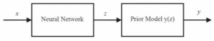
Serial semi-parameterization
A semi-parametric model consists of a prior parametric model with a fixed structure derived from either first principles, existing empirical correlation or mathematical transformation. The second part is a nonparametric model connected in series, such as a neural network, which estimates the intermediate variables to be used in the parametric model. A schematic diagram is shown in Fig. 3.
Figure 3. Schematic of serial semi-parameterization
Parallel semi-parameterization
A parallel semi-parametric model is based on the same concept as the previous approach, but the outputs of the neural network and the parametric model are combined to determine the total model output. The neural network is trained on the residual or the incremental variations between the data and the parametric model to compensate for any uncertainties due to the inherent process complexity. Because the neural networks operate over a much reduced range of output variations, the problem of generalization is not so severe since the input/output ranges
are the same. A schematic diagram is shown in Fig. 4.
Figure 4. Schematic of parallel semi-parameterization
The above two approaches can be combined together to produce a ‘‘hybrid’’ semi-parametric model as shown in Fig. 5. The default parametric model compensates for sparse data and improves extrapolation, the neural network compensates for uncertainty, and the bias of the default model and the parametric output model enforces equality constraints upon the output.
In this study, a serial semi-parameter model was used for predicting the total resistance of milk ultrafiltration.
Figure 5. ‘‘Hybrid’’ semi-parametric model
3- Experimental setup
3-1- Membrane system
Iranian Journal of Chemical Engineering, Vol. 5, No. 2 9 CP layer Cake layer rf R if R m R Membrane Permeation flux 0.33 m2. The two pressure gauges measured
the pressure at the inlet (Pi) and outlet (Po) of the module. These gauges were positioned as close to the inlet and outlet of the membrane as physically possible. A temperature probe was attached to the feed tank and used for monitoring temperature during each run. The tem-perature of the feed was continuously controlled by heat exchanger. An electronic balance and a container were used to record the weight of permeate every 30s for its flux calculation.
3-2- Fouling resistances
The transport of pure water through a membrane is by viscous flow. The membrane hydraulic resistance can be described by Darcy’s Law: w w m J TMP R μ
= (6)
where μw is pure water viscosity, Jw is pure
water flux through a clean membrane and TMP is the transmembrane pressure, which can be calculated for a crossflow ultrafiltration as follows:
p o i P P P
TMP= + −
2 (7)
where Pi and Po are inlet and outlet pressures,
respectively, and Pp is filtrate (or permeate) pressure. The total hydraulic resistance (RT)
to permeate flux was calculated by applying the resistance-in-series model (see Fig. 6) or boundary layer-adsorption model as follows:
p p T J TMP R μ
= (8)
where μp is the permeate viscosity and Jp is the permeate flux. In fact, the total hydraulic resistance is the sum of membrane hydraulic resistance and overall fouling resistance. Therefore,
F m T R R
R = + (9)
m p p F R J TMP
R = −
μ (10)
Figure 6. Schematic of resistance in series model
The overall fouling resistance (RF) can be
represented as the sum of the two components on the basis resistance-in-resistance model: resistance-in-resistance due to reversible fouling (Rrf) and resistance due to
irreversible fouling (Rif). The fouling
resistances were determined as:
m wf wf if R J TMP
R = −
μ (11)
if F rf R R
R = − (12)
where μw and Jwf are viscosity and flux of
clean water through a fouled membrane, respectively. At the end of each run, the membrane unit was firstly flushed with distilled water in the same conditions that each run and water flux (Jwf) was measured
10 Iranian Journal of Chemical Engineering, Vol. 5, No. 2
3-3- Experimental procedure
Skim milk powder, used throughout the experiments, was reconstituted in warm distilled water (about 50°C). Twelve kilograms of reconstituted skim milk was prepared for each run. The same batch of dried milk was used in the all experiments to ensure that changes in measured parameters did not result from the variation in milk composition. The heat treatment used for the milk samples before the ultrafiltration process was pasteurization at 72°C for 15 s. The experiments were performed in five groups. Only one of five parameters of MWCO, fat content, pH, temperature, and TMP was varied for any group. All experimental runs were carried out twice and the results averaged. For each set of processing conditions, the feed tank was first recycled with warm distilled water at processing temperature to warm up the system and evaluate the water flux, then it was recycled with the milk sample at a given temperature. The chosen TMP was set by two control valves. The permeate flux and total hydraulic resistance were measured and recorded every 30s. After each run, the membrane unit was cleaned according to the recommendation of the manufacturer and the water flux of the cleaned membrane was measured at the end of the cleaning process. The cleaning procedure stopped when the original water flux was restored, otherwise fouling was not completely removed and the flushing cycle was repeated until the flux returned.
4- Modeling procedure
4-1- Multidimensional neuro fuzzy modeling
In this study, some experimental data of the spiral wound ultrafiltration test rig are used [3, 20]. MATLAB’s fuzzy toolbox version 2.2.1 is used for modeling. The data are extracted from 19 tests of milk ultrafiltration in various operational and physicochemical conditions. The total data set consists of a matrix with 1050 rows and 7 columns, the
first six columns being the inputs of the neuro- fuzzy system and the seventh column being the dynamic flux of permeate, the net’s output. The data set is separated in two, the training data set and testing data set. The data set is divided at random. Two neuro-fuzzy models are established. In the first model, two Gaussian membership functions, and in the second one, three Gaussian membership functions are used for inputs. The schematic of the models is shown in Fig. 7. The models were trained using the training data set, and later tested using the testing data set. For comparing the models, the sum of squared errors (SSE), mean of squared errors (MSE), root mean of squared errors (RMSE), Akaike goodness of fit criterion (AIC) and Schwarz goodness of fit (SIC) [21-23] were calculated using testing and training data sets by Equations 13-17:
∑
− = n j j j p J J SSE 2 exp, , )( (13)
n J J MSE n j j j p
∑
− = 2 exp, , ) ( (14) n J J RMSE n j j j p∑
− = 2 exp, , ) ( (15) n k n SSE AIC log ⎟+2⎠ ⎞ ⎜ ⎝ ⎛
= (16)
n n k n
SSE
SIC log ⎟+ log( ) ⎠
⎞ ⎜ ⎝ ⎛
= (17)
where Jp,j is the estimated permeate flux in
point j, Jexp,j is measured permeate flux from
Iranian Journal of Chemical Engineering, Vol. 5, No. 2 11 4-2- Hybrid physical model
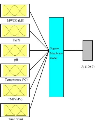
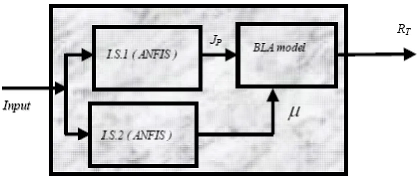
To construct a hybrid physical model, two neuro-fuzzy models are combined with the boundary layer adsorption model to predict total resistance of process in any time. For this purpose, the neuro-fuzzy model with three membership functions is used to predict permeate flux and another neuro-fuzzy model is made to predict viscosity in any time in terms of TMP, temperature, fat% and pH variations. The schematic of this latter model are shown in Fig. 8. The schematic of the complete hybrid model are shown in Fig. 9.
5- Results and discussion
In this work, the application of neuro-fuzzy approach for dynamic prediction of permeate flux decline is tested for ultrafiltration of milk at different physicochemical and operational conditions. The modeling results are presented for flux decline in training and testing stages in Fig. 10 and Table 1. The models 1 and 2 in Table 1 are made with two and three membership functions respectively. Figure 10 illustrates goodness of fit of model 2 for training and testing stages.
Figure 7. Schematic of multidimensional neuro-fuzzy model for predicting permeate flux
MWCO (kD)
Fat %
pH
Temperature (°C)
TMP (kPa)
Time (min)
Jp (10e-6)
Sugeno Membrane model
12 Iranian Journal of Chemical Engineering, Vol. 5, No. 2
Figure 8. Schematic of neuro-fuzzy model for viscosity prediction
Iranian Journal of Chemical Engineering, Vol. 5, No. 2 13
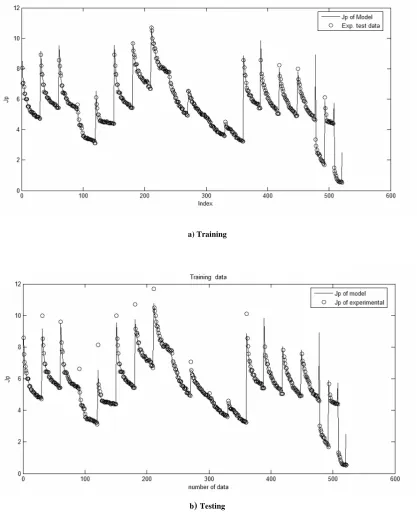
a) Training
b) Testing
Figure 10. Comparison of model results (--) with experimental data (o) for model 2
As shown in Fig. 10a and 10b, there is an excellent agreement between the model predictions (solid lines) and the experimental data (o) of full time-dependent Jp in the training and testing state. Table 1 indicates
the errors of the two models and the criterion of fit goodness, AIC, and SIC. Calculating SSE, MSE and RMSE indicates good results, especially for model 2.
14 Iranian Journal of Chemical Engineering, Vol. 5, No. 2
testing data set
Errors models
Training Testing
SSE MSE RMSE SIC AIC SSE MSE RMSE SIC AIC
Model 1 125.7684 0.2414 0.4913 -0.3647 -1.0835 162.9881 0.3122 0.5588 -0.1054 -0.8243
Model 2 25.945 0.049798 0.22315 6.1857 -0.0631 48.4608 0.0928 0.3047 6.8105 0.5617
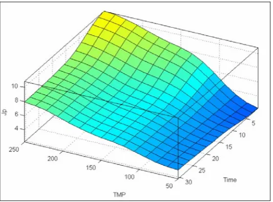
The results of modeling using ANFIS for the permeate flux (Jp) at various transmembrane pressures (TMP) are shown in Fig 11. It can be seen that the magnitude of Jp varies significantly with TMP and time. By increasing the TMP, permeate flux is also increased.
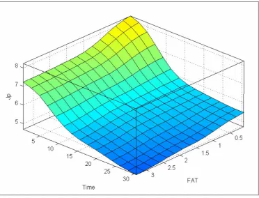
The results of modeling using ANFIS for the permeate flux (Jp) at various temperatures and time are shown in Fig 12. By increasing the temperature, permeate flux is increased. At any time, the steepness is greater in 30°C - 40°C. Optimum temperature is about 40°C. This figure also shows that the complex behavior (non-linearity) of the Jp-time profile is well represented by the ANFIS. The results of modeling using ANFIS for the
permeate flux (Jp) at various fat percentages is shown in Figure 13. It can be seen that by increasing fat percentage, the permeate flux is decreased but the slopes of these decreases are not very great. In the fat percentage of 0.5% to 1.5% the decrease of permeate flux is greater.
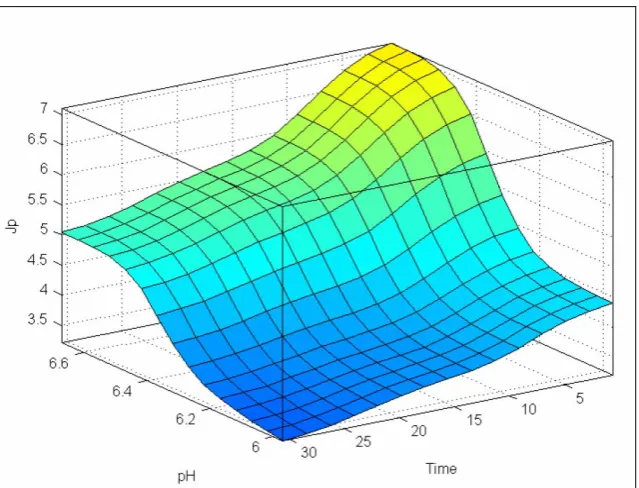
The results of modeling for the permeate flux (Jp) at various pH is shown in Figure 14. It can be seen that, by increasing the pH, the permeate flux is increased. This is because of approaching the isoelectric point of main proteins of milk, which is below pH=5.6 [24], and in the isoelectric point, the solubility of milk proteins is minimum. The present result is the same as the results of other researchers [25, 26].
Iranian Journal of Chemical Engineering, Vol. 5, No. 2 15
Figure 12. Permeate flux as a function of temperature and time. Jp (10e-6) is in m3/m2.s
16 Iranian Journal of Chemical Engineering, Vol. 5, No. 2
Figure 14. Permeate flux as a function of pH and time. Jp (10e-6) is in m3/m2.s
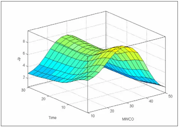
The results of modeling for the permeate flux (Jp) at different MWCO is shown in Fig 15. The variation of permeate flux by various MWCO is paradoxical. At first, by increasing the MWCO the permeate flux is increased, but after MWCO=30, the flux is decreased where the MWCO is increased. This phenomenon happens, probably, because of the alteration of the fouling mechanism in various MWCO. At first, the fouling mechanism is gel-cake formation, and then mechanism changes to pore plugging. The MWCO increase results in the pore size increase, so some macromolecules can penetrate the pores and clog them [27].
For a deeper study a hybrid model is represented too. In this model two of the previous neuro-fuzzy models are combined with a physical model to predict the total resistance of the ultrafiltration process. The results of the hybrid model are presented in Figs 16-20. In Figure 16 the results of modeling for the total resistance are presented in terms of the various TMP and time. It can be seen that, increasing TMP also increases the total resistance. This
phenomenon probably occurs as a result of increased fouling and compaction of the fouling layer.
The results of modeling the variation of total resistance in terms of temperature are shown in Fig. 17. By increasing temperature, total resistance is increased. This is owing to the solubility reduction and denaturation of milk proteins with temperature enhancement in this temperature range. Consequently, fouling is increased, increasing total resistance [28].
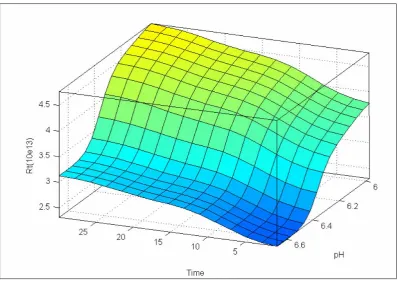
The variations of total resistance versus pH are seen in Fig. 18. Decreasing pH increases total resistance. This is due to increasing concentration polarization and fouling with pH reduction [26, 29-31].
Iranian Journal of Chemical Engineering, Vol. 5, No. 2 17 The results of hybrid modeling for total
residence variation in various MWCO are presented in Figure 20. As shown in the figure, with the variation of MWCO the total
resistance indicates paradoxical variation. This is because of the changing of the fouling mechanism described above.
Figure 15. Permeate flux as a function of MWCO and time. Jp (10e-6) is in m3/m2.s
18 Iranian Journal of Chemical Engineering, Vol. 5, No. 2
Figure 17. Total resistance as a function of temperature and time
Iranian Journal of Chemical Engineering, Vol. 5, No. 2 19
Figure 19. Total resistance as a function of fat% and time
20 Iranian Journal of Chemical Engineering, Vol. 5, No. 2 6- Conclusion
The possibility of using the neuro-fuzzy approach is investigated to predict dynamic permeate flux decline in milk ultrafiltration as a function of operating time, trans-membrane pressure, temperature, pH, fat percentage, and MWCO. Due to the complexity of milk ultrafiltration prediction using conventional methods, these alternative models allow a unified approach that can be used for the analysis of the process and design of new applications.
The modeling results indicate that a complete profile of the milk ultrafiltration performance can be predicted using the ANFIS structure. By increasing the temperature, TMP, and pH the permeate flux is decreased. By increasing the fat percentage, the flux is decreased. The variation of MWCO indicates paradoxical changes in the permeate flux. A model with two-membership functions indicates a better result according to AIC and SIC goodness of fit criterion, but this model’s error is also greater.
For further study, a hybrid physical model for predicting the total resistance of the process is represented. The results indicate that by increasing the TMP, temperature, and fat percentage, the total resistance is increased; but by increasing the pH, total resistance is decreased. The MWCO variation indicates a different total resistance value too.
The future direction of this research is the prediction of permeate flux and total resistance using statistical, physical, and other hybrid models, and then the comparison of the results with these of the present paper.
Acknowledgement
The authors would like to thank Dr. Razavi and the food science department of Ferdowsi University of Mashhad.
Nomenclature
AIC Akaike goodness of fit criterion ANFIS adaptive neuro fuzzy inference
system
f logistic sigmoid activation function
J flux, m3/m2.s
H hidden layer
MSE mean of squared errors MWCO molecular weight cut off, kD
O output
OL output layer
p design parameter (consequent parameter)
q design parameter (consequent parameter)
r design parameter (consequent parameter)
t time, s
T temperature, ◦C
TMP transmembrane pressure, kPa R resistance
RMSE root mean of squared errors SIC Schwarz goodness of fit criterion SSE sum of squared errors
w wiring strength of a rule
W weights
X input
Y target activation of the output layer
Greek symbols
α learning rate
δ error for output neuron
θ threshold between the input and hidden layers
η momentum factor
ρ density, Kg·m-3
µ dynamic viscosity , N·s·m-2
Subscripts
exp experimental F fouling
I input
if irreversible fouling m membrane
o output
Iranian Journal of Chemical Engineering, Vol. 5, No. 2 21 References
1. Perry, R. H., Perry’s Chemical Engineers’ Handbook, Seventh Edition, McGraw-Hill (1999).
2. Cheryan, M., Ultrafiltration and micro-filtration handbook (2nd ed.), Lancaster:
Technomic Publishing Ltd (1998).
3. Razavi, S. M. A., Mousavi, S. M., Mortazavi, S.A., "Dynamic modeling of milk ultra-filtration by artificial neural network," Journal of Membrane Science, 220, 47 (2003).
4. Bowen, W. R., Jones, M. J., Yousef, H. N. S. Dynamic ultrafiltration of proteins-neural networks approach, Journal of Membrane Science, 146, 225 (1998a).
5. Bowen, W. R., Jones, M. J., Yousef, H. N. S. "Prediction of the rate of crossflow membrane ultrafiltration of colloids: A neural network approach," Chemical Engineering Science, 53, 3793 (1998b).
6. Dornier, M., Decloux, M., Trystram, G., Lebert, A., "Dynamic modeling of crossflow microfiltration using neural networks," Journal of Membrane Science, 98, 263 (1995).
7. Delgrange, N., Cabassud, C., Cabassud, M., Durand-Bourlier L., Laine J. M., "Modeling of ultrafiltration fouling by neural networks," Desalination, 118, 213 (1998).
8. Zadeh, L. A., "Fuzzy sets," Information and Control, 8, 338 (1965).
9. Mamdani, E. H., Assilian, S., "An experiment in linguistic synthesis with a fuzzy logic controller," Int. J Man–Machine Stud, 7(1), 1 (1975).
10.Takagi, T., Sugeno, M., "Fuzzy identification of systems and its applications to modeling and control, IEEE Transactions on Systems," Man, and Cybernetics, Marseille, France, 1, 116 (1985).
11.Jang, J. S. R., Gulley, N., "Fuzzy logic toolbox user’s guide for use with MATLAB," Copyright by the Math Works Inc (1999). 12.Wang, L. X., "Adaptive fuzzy systems and
control," Prentice-Hall, Englewood, NJ (1994).
13.Venkatasubramanicon, V., McAvoy, T. J. "Neural network applications in chemical engineering," Computers and Chemical Engineering, 19(4), 1 (1992).
14.Bowen, W. R., Jones, M. J., Welfoot, J. S.,
Yousef, H. N. S., "Predicting salt rejections at nanofiltration membranes using neural networks," Desalination, 129, 147 (2000). 15.Jang, J. S. R., "Fuzzy modeling using
gene-ralized neural networks and Kalman filter algorithm," Proc. of the Ninth National Conf. on Artificial Intelligence, 762-776 (1991). 16.Jang, J. S. R., Sun, C. T., "ANFIS:
Adaptive-network-based fuzzy inter-ference system," IEEE Transactions on Systems, Man, and Cybernetics, 23, 665 (1993).
17.Jang, J. S. R., Sun, C. T., "Neuro-fuzzy modeling and control," Proceedings of the IEEE, 83, 3, 378 (1995).
18.Thompson, M. L., Kramer, M. A., "Modelling chemical processes using prior knowledge and neural networks," AIChE Journal, 40(8), 1328 (1994).
19.Brown, M., Bossley, K. M., Harris, C. J., "The theory and implementation of the B-spline neurofuzzy construction algorithms," EUFIT 96, 2:762 (1996).
20.Razavi, S. M. A., Mousavi, S. M., Mortazavi, S. A., "Application of neural networks for crossflow milk ultrafiltration simulation," International Dairy Journal, 14, 69 (2004). 21.Akaike, H., "Information theory and an
extension of the maximum likelihood principle," Second International Symposium on Information Theory, Akademiai Kiado, Budapest, 267-281 (1973),.
22.Akaike, H., "A new look at the statistical model identification," IEEE Transactions on Automatic Control, 19, 6 (1974).
23.Bierens, H. J., "Information Criteria and model selection," Pennsylvania State University (2004).
24.Fox, P. F., "Advanced dairy chemistry – 1: proteins," Elsevier (1992).
25.Patel, R. S., Reuter, H., "Fouling of hollow fiber membrane during ultrafiltration of skim milk," Milchwissenschaft, 40 (12), 731 (1985).
26.Eckner, K. F., Zottola, E. A., "Effects of temperature and pH during membrane concentration of skim milk on fouling and cleaning efficiency," Milchwissenschaft, 48 (4), 187 (1993).
22 Iranian Journal of Chemical Engineering, Vol. 5, No. 2 28.Ipaktchi, M., "General biochemistry," Vol. 1,
Publication No. 64, Mashhad University Press (1979).
29.Eckner, K. F., Zottola, E. A., "Partitioning of skim milk components as a function of pH, acidulant, and temperature during membrane processing, "Journal of Dairy Science, 75 (8), 2092 (1992).
30.Attia, H., Bennasar, M., Lagaude, A., Hgodot, B., "Ultrafiltration with a microfiltration membrane of acid skimmed and fat-enriched milk coagula: hydrodynamic, microscopic, and rheological approaches," Journal of Dairy Science, 60 (2), 161 (1993).