Volume 59, 2019, Pages 18–33
Proceedings of Pragmatics of SAT 2015 and 2018
Predicting SAT Solver Performance on Heterogeneous
Hardware
Zack Newsham, Vijay Ganesh, and Sebastian Fischmeister
University of Waterloo, Canada
Abstract
In recent years, a lot of effort has been expended in determining if SAT solver per-formance is predictable. However, the work in this area invariably focuses on individual machines, and often on individual solvers. It is unclear whether predictions made on a specific solver and machine are accurate when translated to other solvers and hardware. In this work we consider five state-of-the-art solvers, 26 machines and 143 feature instances selected from the 2011 to 2014 SAT competitions. Using combinations of solvers, machines and instances we present four results: First, we show that UNSAT instances are more pre-dictable than corresponding SAT instances. Second, we show that the number of cores in a machine has more impact on performance than L2 cache size. Third, we show that instances with fewer reused clauses are more CPU bound than those where clause reuse is high. Finally, we make accurate predictions of solution time for each of the instances considered across a diverse set of machines.
1
Introduction
Despite the focus, within the SAT community, on determining the predictability of SAT in-stances, there are few works concerning the effectiveness of predictions made on one machine when executing instances on a second machine. This has led to two problems. First, any tools that make predictions of solver performance can only make them based on instances that have been solved on the same machine the predictions are to be valid on. Secondarily, it is virtually impossible to compare results of past publications in this field without first repeat-ing the experiments on the same hardware. Cross machine models will enable practitioners to make predictions of solver performance on new hardware without first having to run known benchmarks, reducing overall effort. Additionally, if it is possible to determine an “absolute” solution time for an instance — regardless of hardware used — it will be possible to combine benchmarking data from multiple sources. This will allow larger, more comprehensive studies of SAT solver performance to be undertaken without duplication of effort.
2
Experimental setup
The experiments included here were run on the Datamill [1] platform. Datamill is designed to
properties on execution. All machines on the Datamill platform run Gentoo Linux with kernel version 3.3.8, and GCC 4.5.3. A full listing of the machines used is available in Appendix A.
Due to memory constraints within the different machines, and timing constraints for data gathering, it was not possible for every machine, instance, solver combination to complete successfully. To mitigate any bias this may cause in our analysis, we limit ourselves to the set of machines, instances and solvers such that every machine solved every instance in the set on at least one solver. This reduced the number of trials (individual combinations of solvers, machines and instances) available for analysis from 15 588 to 13 648. The number of machines reduced to 21 while the number of instances remained unchanged.
For each machine-based parameterpx and instancei, we used a standard linear regression
with Equation1to calculate the adjustedR2valueri,px for all trialstusing the instancei. As
such, the valueri,pxexpresses the amount of variability in solution time of instanceiaccounted
for by factorpx. The adjustedR2metric ranges from zero to one, with one being a perfect model
and zero indicating that the provided model does not explain the response variable (time). For
brevity, the remainder of this document will use the notationtime∼pin place of Equation1.
timet∼β0+β1px,t+t (1)
We then consider different instance based characteristicscy to determine whether classes of
instances (identified as having similarcyvalues for specified values ofy) are more or less reliant
on different machine parameters.
In total, we considered 34 instance characteristics and 7 machine parameters. While not all of them were found to be significant, those that were are discussed in this work. The machine parameters considered were: CPU speed, CPU architecture, CPU manufacturer, CPU cores, FSB speed, RAM size and L2 cache size. In the future, we intend to increase this set of features, particularly concerning cache sizes and RAM speeds. However, this information is not available for the machines at this time. Modern CPU’s express their FSB speed in GT/i whereas older CPUs utilise MHz. GT/i is considered a more accurate measurement, which describes not only the clock speed of the bus but the data width. As such, we converted all measurements of FSB speed to GT/i. We included CPU Model to determine if CPUs from different models/manufacturers with similar specifications perform differently. A reason for this could be cache replacement policies and implementation specific timing characteristics, such as the proportion of integer vs floating point cores within the CPU. The data in this paper
is available online [2].The instance characteristics considered are listed in Appendix B.
The five solvers considered were MiniSAT 2.0 [3], Glucose 3.0 [4], Lingeling [5], Plingeling
[6] and SWDiA5BY 2.3. These were the silver and gold medal winners of the 2013/2014 SAT
competitions for the application category. While PeneLoPe was also a medal winner, it was excluded as it did not compile on the target environment.
We randomly selected instances from the 2011 to 2014 SAT competitions for these exper-iments. They were selected using a stratified random sampling technique to ensure that we included a diverse set of instances in the sample. The stratified sample considered values of Q,
|Co|, |V|, |Cl|, CVR and solution time. At most three instances were selected for each range
of the measured property.
Prior to running the experiment, we expected that memory size, CPU clock speed and cache
size were going to be significant contributing factors. However, as shown in [7] memory layout
as well as other factors can have a significant impact on any execution times, including that of
a SAT solver. It was for this reason we decided to utilise DataMill [1].
Due to the heterogeneous nature of the hardware used, it was not possible to run all solvers on all machines. We found that the ARMV7 machines (machines 22-25 in Appendix A) were only able to run Lingeling. All the other solvers (including pLingeling) failed to compile due to a floating point library not being present in the ARM version of the operating system. Each machine was dedicated to running only the experiment given and is not virtualised or shared in any way.
To remove the possibility that these timing differences were the result of randomness in the solver, we pre-simplified the instances then turned off simplification on the solvers. This is to
resolve the known issue that clause (and variable) ordering has an effect on solution time [8].
In addition to this we set a fixed random seed for all the solvers on all machines (with the exception of pLingeling that did not support this option). In doing so, we ensure that a single instance/solver pair should have identical performance on an identically specified machine.
The complete set of all combinations of solvers, workers and instances would have created approximately 18 500 trials. Unfortunately even with the time-outs and batching we imposed, DataMill was unable to complete all of these trials within the required time frame. As such we are limited to analysing those results which were gathered, approximately 15 500 of them. Within these results approximately 1 600 were unable to run due to a lack of support in the ARM kernel, as mentioned previously. Leaving a total of 13 825 instances available for analysis. The majority of our analysis looks at aggregate results, either across the instances, solvers or workers. We only analysed the complete set of workers and instances, by which we mean that every worker in our final dataset solved every instance at least once. We chose to do this to ensure that no bias has been introduced by certain combinations of workers/instances not completing. To accomplish this we used an implementation of maximal biclique enumeration
algorithm from Alexe et al [9] where the workers are one half of the graph and the instances
are the other. The resulting clique included 13 648 trials. Unless otherwise stated this is the
set used in all results presented. Similarly, unless otherwise stated,timerefers to the wall clock
time.
3
Results
The following sections detail the results mentioned above. In each of the four sections we discuss a single result, providing evidence and levels of confidence of it, and discuss the consequences of that result.
3.1
UNSAT instance performance is more predictable than SAT
When analysing the set of all trials, regardless of solver, a clear trend can be observed re-garding the predictability of instances. For all machine parameters considered, UNSAT in-stances were consistently more predictable than SAT inin-stances. For example, using the model
time∼CP U Speed the maximum R2 for UNSAT instances is 0.65, whereas the maximum R2
for SAT instances is 0.64. While, in this case, the maximum R2 does not differ significantly,
17.4% of the 69 UNSAT instances had an R2>0.5 and 55.0% had an R2>0.3. This is
com-pared with SAT instances, where only 4.0% of the 74 SAT instances had an R2>0.5 and 24.3%
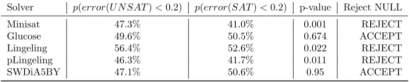
Solver p(error(U N SAT)<0.2) p(error(SAT)<0.2) p-value Reject NULL
Minisat 47.3% 41.0% 0.001 REJECT
Glucose 49.6% 50.5% 0.674 ACCEPT
Lingeling 56.4% 52.6% 0.022 REJECT
pLingeling 46.3% 41.7% 0.011 REJECT
SWDiA5BY 47.1% 50.6% 0.95 ACCEPT
Table 1: Shows the probability that a prediction error for an instance using the model
time CP U Speedwill be less than 20% of that instances execution time. The p-value column shows the significance level of the test.
Previous results [10] have shown that UNSAT instances have more predictable performance,
when considering different instances on the same hardware. However, our result focuses on the predictability of the performance of individual UNSAT instances across a diverse set of hardware.
The same trend, of UNSAT instances having a higher R2 score, can be observed for FSB
speed, RAM size, L2 size and number of CPU cores. Though it should be mentioned that SAT
instances achieved a marginally higher maximum R2 for L2 size (0.14) compared to UNSAT
instances (0.13). However, fewer SAT instances achieved anR2>0.05 than UNSAT.
Further results in Section3.4support the result that UNSAT instance performance is more
predictable than SAT instance performance. To demonstrate this, we test the following
hy-pothesis, whereS is the set of solvers described in Section2:
H1s,0:p(error(U N SATs)<0.2)≤p(error(SATs)<0.2), ∀s∈S
H1s,a:p(error(U N SATs)<0.2)> p(error(SATs)<0.2), ∀s∈S
The functionpreturns the probability that the predictions for the set of instances provided
will be accurate to with 20% of the solution time of each instance. We then utilise a binomial probability test to determine whether the probability of an accurate prediction is higher for UNSAT instances than SAT, for each solver.
We performed the hypothesis test with a significance level of 0.05, as such we accept the
null hypothesis in the cases where the p-value>0.05. Table1shows the results of this
hypoth-esis test. Each row in the table presents the result of the hypothhypoth-esis test for a single solver, along with the probabilities of accurate predictions for the SAT and UNSAT instances on that solver, and finally whether we accept or reject the null hypothesis. For MiniSAT, Lingeling and pLingeling, UNSAT instances are more predictable than SAT instances, with a p-value low enough that we reject the null hypothesis. However, in the cases of Glucose and SWDiA5BY, the results suggest that SAT instances are more predictable than UNSAT. It is unclear why Glucose and SWDiA5BY should show a different result than the other solvers and requires further experimentation at a later date.
3.2
Number of cores is more important than L2 cache size
Solver p(L2>0.1) p(CP U Cores >0.1) p-value Reject NULL
MiniSAT 12.6% 94.4% <0.001 REJECT
Glucose 12.6% 96.5% <0.001 REJECT
Lingeling 3.5% 35.0% <0.001 REJECT
pLingeling 65.0% 95.0% <0.001 REJECT
SWDiA5BY 18.9% 98.6% <0.001 REJECT
Table 2: The results of the hypothesis test H2, showing the probability that the R2 for the
modelstime∼L2>0.1 andtime∼CP U Cores, as well as the p-value for the hypothesis test
thatCP U Cores > L2
The maximum R2 for the modeltime∼L2 was 0.14, compared with the maximum R2for
the modeltime∼CP U Cores which was 0.57.
To confirm the result that the number of cores is more important in determining solver
performance than L2 cache size, we test the following hypothesis. S is the set of solvers
described in Section 2 and the function p returns the probability that the provided machine
parameters R2 will exceed 0.1:
H20,s:p(L2s>0.1)≤p(CP U Coress>0.1), ∀s∈S
H2a,s:p(L2s>0.1)> p(CP U Coress>0.1), ∀s∈S
Table 2 shows, for each solver, the probability that the value of R2 will exceed 0.1 for
the model time∼L2. The probability that the value of R2 will exceed 0.1 for the model
time∼CP U Cores. The p-value for the hypothesis test and whether we reject or accept the null hypothesis. In every case, the solver’s performance is impacted significantly more by the number of CPU cores than the L2 cache size.
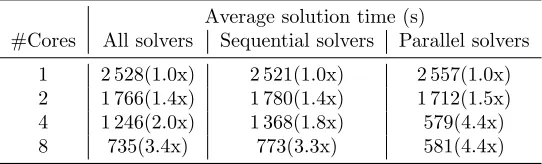
One possible explanation for this result is the overall trend between both CPU speed and number of cores, and RAM size and number of cores. However, there are several machines that do not follow this trend (E.g., machines number 3,7 and 20). Another possible explanation for this result is that L2 cache size is not representative of the overall impact of cache size on solver performance. The L1 cache and lowest level cache (which in some cases will be L2) are potentially more significant than L2 cache size alone. The reason for excluding the L1 and “lowest level” cache sizes is that, at present, we do not have that data for all machines considered. This will be included in future versions of this work. A third possible explanation for the performance increase is that overhead in the operating system takes place on one core,
while the solving of the SAT problem takes place, uninterrupted, on another. Table3 shows
Average solution time (s)
#Cores All solvers Sequential solvers Parallel solvers
1 2 528(1.0x) 2 521(1.0x) 2 557(1.0x)
2 1 766(1.4x) 1 780(1.4x) 1 712(1.5x)
4 1 246(2.0x) 1 368(1.8x) 579(4.4x)
8 735(3.4x) 773(3.3x) 581(4.4x)
Table 3: Number of cores and the associated average execution time in seconds, the bracketed number is the speedup relative to single core performance.
c1: 1 2 3 0
c2: -1 2 3 0
c3: 1 3 -4 0
c4: 1 -2 3 0
3.3
A negative correlation exists between clause reuse and the impact
of CPU speed on solver performance
In this section we use the term “clause reuse” to indicate sets of clauses with the same variables with different polarity. For example, in the DIMACS below clause c1 is said to be reused two times (in clauses c2 and c4). Clause c3 is seen only once (clause reuse of 0).
The terms max(reuse) and mean(reuse) refer to the maximum and average times any single
clause is reused. Figures 1a and 1b show, for SAT and UNSAT instances respectively, the
correlation between the average clause reuse for formula (on the x-axis) and the average R2of
the modeltime∼CP U Speedfor those instances (on the y-axis). Each data point represents a
0.1 range of the average clause reuse.
Figures 1a and 1b show a negative correlation between the average clause reuse and the
impact of CPUSpeed as a predictor of time. This negative correlation indicates that instances, where individual clauses contain unique sets of variables, are more CPU bound than those which have a small set of variables that are repeatedly assigned different values in clauses.
To confirm this result, we test the following two hypothesis, where S is the set of solvers
described in Section2:
H30,s:p(time(il, s))≤p(time(ih, s)), ∀s∈S, M ean.Reused(il)< M ean.Reused(ih)
H3a,s:p(time(il, s))> p(time(ih, s)), ∀s∈S, M ean.Reused(il)< M ean.Reused(ih)
Functionpreturns the predictability of the execution time of a solver on a particular instance
across all considered hardware. ihandil refer to randomly selected instances with higher, and
lower average clause reuse respectively.
For this experiment, we randomly selected 500 pairs of instances and checked whether the instance with the lower mean(reused) value was more CPU bound than the instance with the
higher mean(reused). Table 4 shows the probability that for any randomly selected pair of
instances (where the mean(reused) differ) the alternate hypothesis holds true. It also shows the significance level of the test, and whether we accept or reject the null hypothesis.
For all solvers, with the exception of MiniSAT, we reject the null hypothesis. This confirms
the visual result presented in Figures 1a and 1b, the more frequently a clause is reused, the
●
● ●
●
● ●
●
● ●
●
● ●
●
●
0.0 0.5 1.0 1.5 2.0 2.5 3.0
0.00
0.05
0.10
0.15
0.20
0.25
Effect of CPU speed on time WRT mean(reused)
mean(reused) Rcpu
2
● SAT
(a) For SAT instances
● ●
● ●
● ●
●
● ● ●
●
●
●
0 2 4 6 8 10 12 14
0.05
0.10
0.15
0.20
0.25
0.30
0.35
0.40
Effect of CPU speed on time WRT mean(reused)
mean(reused) Rcpu
2
● UNSAT
(b) For UNSAT instances.
Figure 1: Figures showing the clause reuse against average R2 for SAT and UNSAT instances,
the line represents the moving average over a window of seven data points.
Solver %H3a holds p-value Reject NULL
MiniSAT 50.0% 0.954 ACCEPT
Glucose 61.0% 0.001 REJECT
Lingeling 63.4% 0.001 REJECT
pLingeling 63.6% 0.001 REJECT
SWDiA5BY 63.4% 0.001 REJECT
Table 4: Shows the results of the hypothesis test H3. For each solver the % of randomly selected
pairs of instances where H3a holds is given, along with the p-value of the hypothesis test.
need to consider the specification of the hardware, but also characteristics of the instance. It is not clear why MiniSAT does not exhibit the same pattern as the other solvers considered, this is a subject we are considering for future work.
3.4
Predicting performance
Using a standard linear regression with Equation2we can predict the solution time of individual
instances on specific solvers for previously untested hardware, based on their performance on
our test machines. This model results in an R2>0.73 for 80% of the instances considered,
across all solvers. The⊕notation here denotes that not only were each of the individual factors
considered but all interaction terms of the three factors as well.
timeis∼CP U Speed⊕CP U Cores⊕RAM (2)
Solver Median error (s) Maximum error (s) 80% error (s)
MiniSAT 104 163894 1087
Glucose 53 1939631 665
Lingeling 46 1218864 555
pLingeling 89 2116591 999
SWDiA5BY 50 111689 641
Table 5: The predictability of different solvers, showing median, maximum and the 80% confi-dence level of predictions, for each of the considered solvers.
solver, where 80% of instances had an R2>0.87. SWDiA5BY and MiniSAT were the least
predictable solvers, where in both cases 80% of instances had an R2>0.80. This indicates
that Lingeling’s performance is less determined by factors not included in our model, such as RAM speed and cache sizes. Conversely, the performance of MiniSAT and SWDiA5BY may be effected by these absent parameters.
To test these results, we performed a k-fold cross validation with k= 5. For each instance
and solver combination, we randomly partitioned the machines into five equal partitions. Four of these are used as a training set to predict the execution time of the machines from the
one remaining partition. We repeated the analysis using the same partitioning five times,
using a different partition as the test partition each time. We repeated this entire process ten times for each solver, with different randomly created partitions to mitigate the issue of different prediction error depending on which machines were assigned to the training and test
sets. Table 5shows the predictability of the five considered solvers according to their median
absolute error, maximum error and 80% confidence level. This data confirms that predictions made for the Lingeling solver are most accurate, and that predictions made by MiniSAT are least accurate. However, SWDiA5BY predictions were relatively accurate, while pLingeling predictions were significantly less accurate.
This is indicated by the increased median error and 80% confidence level. The difference between MiniSAT and pLingeling in this case is small, fifteen seconds for the median error and 88 seconds for the 80% confidence level. One possible explanation is that machines were assigned to folds randomly, as such it is possible that the assignment for the MiniSAT instances was less predictive than the one used for pLingeling.
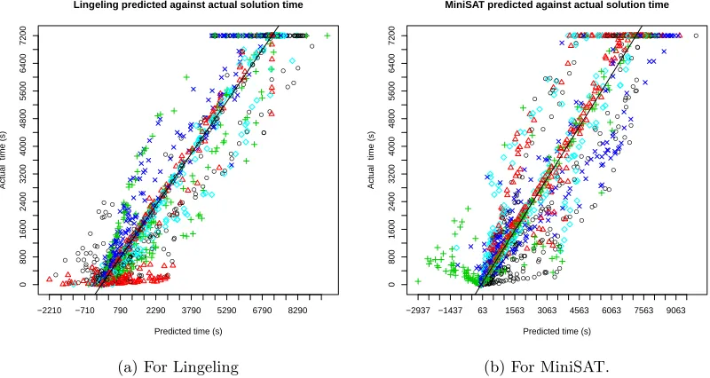
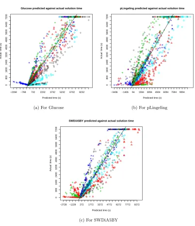
Due to the random sampling performed, results vary on depending on which machines are
assigned to each fold for the cross-validation. Had we setk= 21 this would not have been the
case. However, one of our goals is to find a small subset of machines that can be used to predict solution times across a wide range of hardware, as such we were interested in minimising the
training set. Figures2aand2bshow the results of the cross validated predictions for Lingeling
and MiniSAT respectively. These solvers are highlighted as they were the most and least
predictable solvers respectively.
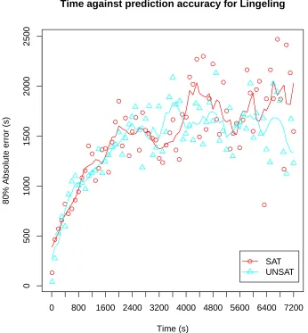
Unfortunately, no obvious trend exists between the quality of the predictions, and any of the 34 considered instance characteristics. However, there does exist a trend between the quality
of the predictions, and the average execution time for the instances. Figure3shows the trend
● ● ● ● ● ● ● ● ● ● ● ● ● ● ● ● ● ● ● ● ● ● ● ● ● ● ● ● ● ● ● ● ● ● ● ● ●● ● ● ● ● ● ● ● ● ● ● ● ● ● ● ● ● ● ● ● ● ● ● ● ●●● ● ● ● ●●●● ● ● ● ● ● ● ● ● ● ● ● ●●●●●●●●●●●●●●●●●●● ● ●● ● ● ● ● ● ● ● ● ● ● ● ● ● ● ● ● ● ● ●● ●●● ● ● ● ● ● ● ● ● ● ● ● ● ● ● ● ● ● ● ● ● ● ● ● ● ● ● ● ● ● ● ● ● ● ● ● ● ● ● ● ● ●●●●●●●●●● ●●●● ● ● ● ● ● ● ● ● ● ● ● ● ● ● ● ● ● ● ● ● ● ● ● ● ● ● ● ● ● ● ● ●●●●● ● ● ● ● ● ● ● ● ● ● ● ● ● ● ●● ● ● ● ●● ● ● ● ● ● ● ●●● ● ● ● ● ● ● ● ● ● ● ● ● ● ● ● ● ●●●●● ● ● ● ● ● ● ● ●●●●● ●●●● ● ● ● ● ● ● ● ● ● ● ● ●● ●● ●●● ● ● ● ● ● ● ● ● ● ● ● ● ●●●●● ● ● ● ●● ●●●●● ● ● ● ● ●● ● ● ● ● ● ● ● ● ● ● ● ● ● ● ● ● ● ● ● ● ● ● ● ● ● ● ● ● ● ● ● ● ● ● ● ●●●●●●●●●● ● ● ● ● ● ● ● ● ●● ● ● ● ● ● ● ● ● ● ● ● ● ● ● ● ● ● ● ● ● ● ● ● ● ● ● ● ● ● ● ● ● ● ● ● ●● ● ● ● ●●●●● ● ● ● ● ● ● ● ● ● ● ● ● ● ●●●●● ● ● ● ● ● ● ● ● ● ● ● ● ●● ●●●●● ●●●●●●●●●● ● ● ● ● ● ● ● ● ● ● ● ● ● ● ● ● ● ● ● ● ● ● ● ●● ●●●●●●●● ●●●●● ●●●●●●●●● ● ● ● ● ● ● ● ● ● ● ● ● ● ● ● ● ● ● ● ● ● ● ● ●● ● ● ● ● ● ● ● ● ● ● ● ● ●●●●● ● ● ● ● ● ● ● ● ● ● ● ● ● ● ● ● ● ● ● ● ● ● ● ● ● ● ● ● ● ● ● ● ● ● ● ● ● ● ● ● ● ● ● ● ● ● ● ● ● ● ● ● ● ● ● ● ● ● ● ● ● ● ● ● ● ● ● ● ● ● ● ● ● ● ● ● ● ●● ● ● ● ● ● ● ● ● ● ● ● ● ● ●●●
Lingeling predicted against actual solution time
Predicted time (s)
Actual time (s)
0 800 1600 2400 3200 4000 4800 5600 6400 7200
−2210 −710 790 2290 3790 5290 6790 8290
(a) For Lingeling
● ●● ● ● ● ●●● ● ● ● ● ● ● ● ● ● ● ● ● ● ● ● ● ● ● ● ● ● ● ● ● ● ● ● ● ● ● ● ● ● ● ● ● ● ● ●●●●●● ● ● ● ● ● ● ● ● ● ● ● ●● ●●● ● ● ● ● ● ● ● ● ● ● ● ● ● ● ● ● ● ● ● ● ● ● ● ● ● ● ● ●●●●●●●● ● ● ● ● ● ● ● ● ● ● ● ● ● ● ● ● ● ● ● ● ● ● ●●● ● ● ● ● ● ● ● ● ● ● ● ● ● ● ● ● ● ●●● ● ● ● ●●●● ● ● ●● ●●● ● ● ● ● ● ● ● ● ● ● ● ● ● ● ● ● ● ● ● ● ● ● ● ● ● ● ● ● ● ● ● ● ● ● ●● ● ● ● ●● ● ● ● ● ● ● ● ● ● ● ● ● ● ● ● ● ● ● ● ● ● ● ● ● ● ● ● ● ● ● ● ● ● ● ● ● ● ● ● ● ● ● ● ● ● ● ● ● ● ●●● ● ● ● ● ● ● ● ● ● ●●● ● ● ● ● ● ● ● ● ● ● ● ● ● ● ● ● ● ● ● ● ● ●● ● ● ● ●● ● ● ● ● ● ● ● ● ●●● ● ● ● ● ●● ● ● ● ● ● ● ● ● ● ● ● ● ● ● ● ● ● ● ● ● ● ● ● ● ● ● ● ●●●●● ● ●● ●●●●●●●●●●● ● ● ● ● ● ● ● ● ● ● ● ● ● ● ● ● ● ● ● ● ● ● ● ●● ● ● ●●●●●●●●● ● ● ● ● ● ● ● ● ● ● ● ● ● ● ● ● ● ● ● ● ● ● ● ● ● ● ● ● ● ●●● ● ● ● ● ● ● ● ● ● ● ● ● ● ● ● ● ● ● ● ● ● ● ● ● ● ● ● ● ● ● ● ● ● ● ● ● ● ● ● ● ● ● ● ● ● ● ● ● ● ●● ● ● ● ● ● ● ● ● ● ● ●● ● ● ● ● ● ● ● ●
MiniSAT predicted against actual solution time
Predicted time (s)
Actual time (s)
0 800 1600 2400 3200 4000 4800 5600 6400 7200
−2937 −1437 63 1563 3063 4563 6063 7563 9063
(b) For MiniSAT.
Figure 2: Figures showing the predicted solution times against actual solution times for the Lin-geling and MiniSAT solvers for a single repetition of the k-fold cross validation. Approximately 5% of the outlier data points are omitted from these plots to improve interpretability. The different colours represent the individual folds. The black line represents perfect predictions.
instances in this dataset timeout, of those instances, 42% were on UNSAT instances and 58% were on SAT instances. Considering the UNSAT instances show more accurate predictions over the increasing range of execution time and have fewer timeouts, when compared to SAT instances, this would support our conjecture.
4
Related Work
The related work falls into two categories. First, there is significant work on predicting SAT solver performance on sets of instances, on fixed hardware. Second, there has been significant work outside of the SAT community in the prediction of program execution time on diverse hardware.
In 2010, Kadioglu et al presented a method for instance specific algorithm configuration
(ISAC) [11]. This work, which encompasses algorithm selection and tuning, focused on
char-acteristics of the input instance to tune the selected algorithm and thus increase performance. They utilise g-means to cluster the instances, working on the premise that instances that are clustered together will behave similarly when solving.
In 2012, Malitsky and Sellmann presented the idea of using ISAC for the construction of
portfolio based SAT solvers [12]. They compare this performance against that of portfolio based
solvers, such as SATzilla [13], and show that, in many cases, ISAC outperforms them.
In 2012, an update on SATzilla was published [13] which presented the utilisation of
cost-sensitive classification models. In this version of SATzilla, feature computation is limited to 90 CPU seconds. This is a particularly interesting technique when considering community-based
● ●
● ●
● ●●
● ●
● ●
● ●
● ●
●●
● ●
● ●
● ●
● ●
●
● ●
●● ●●
● ●
● ●
●
● ●
●● ●
● ●
● ●
● ●
●
●
● ●
●
● ●
●
● ●
●
●
● ●
●
● ●
●
● ●
●
● ●
●
●
Time against prediction accuracy for Lingeling
Time (s)
80% Absolute error (s)
0
500
1000
1500
2000
2500
0 800 1600 2400 3200 4000 4800 5600 6400 7200
● SAT
UNSAT
Figure 3: The correlation between the 80% confidence level for predictions, and the average solution time of the instances. The lines represent the moving average over a window of five data, each data point represents a 10 second time interval.
high, when compared to a relatively low execution times of a solver on certain types of instance. In 2004, Marin and Mellor-Crummey presented a work on predicting parallel application
performance across different architectures using parametrised models [15]. In this work, the
authors utilise instrumented code to predict execution times, considering factors such as the execution count of individual sequential sections of code and memory latency on the target architecture. This technique requires measuring specific hardware factors (such as the cost of an L1 cache miss) at execution times to enable accurate predictions.
using partial execution [16]. This technique utilises observation based techniques and as such has no need to consider features of the platform, such as CPU speed, memory size, etc. The advantage of this technique is that it can be highly accurate for certain types of program, it is unclear whether SAT solvers fall into this category. However, one drawback is, that for each new platform, a representative set of sample applications must be ran for the predictions to be accurate. This makes the technique more valid for large-scale parallel computing clusters that utilise multiple instances of similarly specified hardware.
In 2006, Hoste et al presented a work on predicting application performance based on
program simplicity [17]. This work utilises the SPEC CPU2000 [18] results on 36 machines
to determine if a correlation exists between the proposed simplicity metrics and the speedup rates published in SPEC CPU 2000. Their results show an improved worst-case and average correlation coefficient when compared to current practice.
In 2006, Lee and Brooks presented a work on predicting application performance on the
Turandot simulator [19]. They consider 12 architectural parameters including the number of
general purpose registers, sizes of L1 and L2 cache, and memory and L2 latency. The use of a simulator allowed high levels of control on features such as pipeline depth and memory latency in cycles. They found that application specific models were most predictive of performance prediction.
5
Conclusion
In this work, we have explored the relationship between different classes of instances, and their solution times on differently specified machines and solvers. We have shown that the solution time for a specific instance varies greatly across different machines, in ways that are not completely predictable when considering characteristics such as CPU speed, RAM size and cache size. We have further shown that the impact of each of these factors on the solution time of an instance depends on the structure of the instance. In some cases, this structure is characterised by graph theoretical concepts, and others use SAT specific concepts such as the clause-variable ratio.
We have presented a model that can predict the solution time of SAT instances across a diverse set of hardware with relatively high accuracy. We have also identified that, of the observed solvers, Lingeling has the most predictable performance and UNSAT instances are gen-erally more predictable than SAT instances. In addition to the results presented here, we have found strong correlations between the predictability of instance performance and max(reused), max(clause), mean(clause), max(var) as well as others. These results are omitted from this work for the sake of brevity.
While we have not been able to produce a model that completely explains the variability in solution time when varying the machines, we have been able to explain a large amount of it. The remaining variability is likely to be in the factors that were only partially available in our dataset (e.g. cache sizes, RAM speeds, etc). However, we also speculate that cache replacement policies will be a determining factor in solution times of specific instances.
6
Future Work
issue of un-defined variation. However, if this does not complete the model we are planning on exploring the relationship between cache replacement policies and performance. We feel this may be what is missing when we compare machines with different specifications, which perform similarly — for example, the Pentium M and Pentium D machines as described above.
While it was important to perform a fair random assignment for the k-fold cross validation, we also intend to perform a “cherry-picked” version where we select individual machines based on their parameters as the training set. In doing so, we hope to maximise the quality of our predictions while minimising our training set.
In this work, we chose to perform the analysis with a standard linear regression, and it has provided some strong results. However, it is not the only analysis technique suitable for
this area. Random forests [20], non-linear regression and Bayesian inference are examples of
techniques that have been used with varying levels of success to predict the solution time of sets of instances on fixed hardware. While we are focusing on predicting the solution times on heterogeneous hardware from known solution times, these techniques could also apply.
Finally, we are looking into tuning SAT solvers based on the hardware that is being used to solve an instance. It has already been established that some solvers perform better on different hardware, and different classes of instance. While there has been significant work in
selecting/tuning an algorithm based on instance characteristics [11,12,21,22], there has been
relatively little work in selecting/tuning an algorithm based on the hardware being used.
References
[1] Augusto Oliveira, Jean-Christophe Petkovich, Thomas Reidemeister, and Sebastian Fischmeister. Datamill: Rigorous performance evaluation made easy. InProc. of the 4th ACM/SPEC Interna-tional Conference on Performance Engineering (ICPE), pages 137–149, Prague, Czech Republic, April 2013.
[2] Zack Newsham. Maching parameters experimental data. http://satbench.uwaterloo.ca/ download/55/1, 2014. Accessed: 2015-01-10.
[3] Niklas Een and Niklas S¨orensson. Minisat: A SAT solver with conflict-clause minimization. SAT, 5, 2005.
[4] Gilles Audemard and Laurent Simon. Glucose: a solver that predicts learnt clauses quality. 2009. [5] A Biere. Lingeling.SAT Race, 2010.
[6] A Biere. Plingeling: solver description.SAT Race, 2010.
[7] Augusto Oliveira, Jean-Christophe Petkovich, and Sebastian Fischmeister. How Much Does Mem-ory Layout Impact Performance? A Wide Study. InProceedings of the International Workshop on Reproducible Research Methodologies (REPRODUCE), page 23–28, Orlando, USA, Febuary 2014. [8] Rodrigo Casta˜no and Jos´e M Casta˜no. Propositional satisfiability (sat) as a language problem. In
XVII Congreso Argentino de Ciencias de la Computaci´on, 2011.
[9] et al Alexe. Maximal biclique enumeration implementation. http://genome.cs.iastate.edu/ supertree/download/biclique/README.html, 2004. Accessed: 2015-01-10.
[10] Kevin Leyton-Brown, Holger H Hoos, Frank Hutter, and Lin Xu. Understanding the empirical hardness of np-complete problems.Communications of the ACM, 57(5):98–107, 2014.
[11] Serdar Kadioglu, Yuri Malitsky, Meinolf Sellmann, and Kevin Tierney. Isac-instance-specific al-gorithm configuration. InECAI, volume 215, pages 751–756, 2010.
[13] Lin Xu, Frank Hutter, Jonathan Shen, Holger H Hoos, and Kevin Leyton-Brown. Satzilla2012: improved algorithm selection based on cost-sensitive classification models. Balint et al.(Balint et al., 2012a), pages 57–58, 2012.
[14] Aaron Clauset, Mark EJ Newman, and Cristopher Moore. Finding community structure in very large networks. Physical review E, 70(6):066111, 2004.
[15] Gabriel Marin and John Mellor-Crummey. Cross-architecture performance predictions for scientific applications using parameterized models. InACM SIGMETRICS Performance Evaluation Review, volume 32, pages 2–13. ACM, 2004.
[16] Leo T Yang, Xiaosong Ma, and Frank Mueller. Cross-platform performance prediction of parallel applications using partial execution. InSupercomputing, 2005. Proceedings of the ACM/IEEE SC 2005 Conference, pages 40–40. IEEE, 2005.
[17] Kenneth Hoste, Aashish Phansalkar, Lieven Eeckhout, Andy Georges, Lizy K John, and Koen De Bosschere. Performance prediction based on inherent program similarity. InProceedings of the 15th international conference on Parallel architectures and compilation techniques, pages 114–122. ACM, 2006.
[18] John L Henning. Spec cpu2000: Measuring cpu performance in the new millennium. Computer, 33(7):28–35, 2000.
[19] Mayan Moudgill, John-David Wellman, and Jaime H Moreno. Environment for powerpc microar-chitecture exploration. Micro, IEEE, 19(3):15–25, 1999.
[20] Frank Hutter, Lin Xu, Holger H Hoos, and Kevin Leyton-Brown. Algorithm runtime prediction: Methods & evaluation. Artificial Intelligence, 206:79–111, 2014.
[21] Frank Hutter, Youssef Hamadi, Holger H Hoos, and Kevin Leyton-Brown. Performance prediction and automated tuning of randomized and parametric algorithms. In Principles and Practice of Constraint Programming-CP 2006, pages 213–228. Springer, 2006.
Appendix A
A list of all machines used in the various experiments in this paper.
# CPU Cores CPU speed
Cache (L1 i/d + L2 + L3)
RAM amount
RAM speed
1 Intel Core i7 i686 4 3400 32/32 + 256 + 8192 8266580 0
2 Intel Pentium M i686 1 1695 0/0 + 256 + 0 902287 0
3 Intel Pentium 4 i686 2 2992 0/16 + 2048 + 0 894177 533
4 VIA Nano X2 i686 2 1733 128/128 + 2048 + 0 1814036 1066
5 Intel Pentium 4 i686 2 3200 0/0 + 512 + 0 1000263 0
6 Intel Pentium 4 i686 1 1595 0/0 + 256 + 0 254781 0
7 Intel Pentium 4 i686 2 2998 0/16 + 1024 + 0 893347 0
8 Intel Pentium 4 i686 1 1595 0/0 + 256 + 0 514119 133
9 Intel Pentium 4 i686 2 2992 0/0 + 1024 + 0 894269 0
10 Intel Pentium 4 i686 2 3200 0/0 + 512 + 0 1000540 0
11 Intel Pentium 4 i686 2 2793 64/64 + 2048 + 0 902461 0
12 Intel Pentium 4 i686 2 1614 0/0 + 256 + 0 894269 0
13 Intel Pentium 4 i686 2 1600 0/0 + 256 + 0 242851 0
14 Intel Pentium 4 i686 2 3198 0/0 + 512 + 0 894269 0
15 AMD Athlon XP i686 1 1111 64/64 + 256 + 0 514199 0
16 Intel Pentium D i686 2 2993 0/0 + 1024 + 0 2076180 0
17 Intel Pentium 4 i686 2 3200 0/16 + 512 +0 894269 0
18 Intel Pentium 4 i686 2 3192 0/0 + 512 + 0 505661 0
19 Intel Xeon x86 64 2 3000 0/0 + 4098 + 0 2831155 0
20 Intel Pentium 4 i686 2 3200 0/0 + 512 + 0 2076180 0
21 Intel Core i7 x86 64 8 3401 128/128 + 1024 + 0 8095006 0
22 ARM Rev 10 armv71 4 1988 0/0 + 1024 + 0 896563 0
23 ARM Rev 10 armv71 4 1988 0/0 + 1024 + 0 896563 0
24 ARM Rev 10 armv71 4 1988 0/0 + 1024 + 0 896563 0
25 ARM Rev 10 armv71 4 1988 0/0 + 1024 + 0 896563 0
26 Intel Core i5 x86 64 4 3291 128/128 + 1024 + 0 8095006 0
27 Intel Core i7 64 4 3400 32/32 + 256 + 8192 8388608 0
28 AMD Athlon 1 757 64/64 + 256 + 0 773079 0
Appendix B
The full description of all features considered in this paper.
Variable Name Definition
vars The number of variables in the formula
weight The difference in the number of true/false literals.
CO The set of communities
Q The quality (Q) of the community structure
max(var) The maximum number of times a variable appears
mean(var) The average number of times a variable appears
min(com) The size of the smallest community
mean(com) The average community size
max(com) The size of the largest community
sd(com) The standard dev of the community sizes
min(inter) The minimum number of inter-com edges from one community
max(inter) The maximum number of inter-com edges from one community
mean(inter) The average number of inter-com edges from one community
sd(inter) The standard dev of inter-com edges from one community
min(intra) The minimum number of intra-community edges in one community
max(intra) The maximum number of intra-community edges in one community
mean(intra) The average number of intra-community edges in one community
sd(intra) The standard dev of intra-community edges in one community
edgeratio The overall ratio of inter/intra edges
max(edgeratio) The maximum ratio of inter/intra edges for one community
min(edgeratio) The minimum ratio of inter/intra edges for one community
mean(edgeratio) The average ratio of inter/intra edges for one community
sd(edgeratio) The standard deviation ratio of inter/intra edges for one community
U E The set of unique edges in the graph
T E The set of all edges (counting degrees) in the graph
CL The set of all clauses
V U C The set of clauses using distinct variables
max(clause) The length of the longest clause
mean(clause) The average clause length
max(reused) The maximum times a clause with the same variables is reused
min(reused) The minimum times a clause with the same variables is reused
mean(reused) The average times a clause with the same variables is reused
CVR The ratio of clauses to variables
TVR The ratio of total clauses to clauses using unique sets of variables
Appendix C
● ● ● ● ● ● ● ● ● ● ● ● ● ●● ● ●● ● ● ● ● ● ● ● ● ● ● ● ● ● ● ● ● ● ● ●● ● ● ● ●● ● ●● ●● ● ● ●● ● ● ● ● ● ● ● ● ●● ● ● ● ●●●●● ● ● ● ●● ● ●● ● ● ● ● ● ● ● ● ● ● ● ● ● ● ● ● ● ● ● ● ● ● ● ● ● ● ● ● ● ● ● ● ● ● ● ● ● ● ● ● ● ● ● ● ● ● ● ● ● ● ● ● ● ● ● ● ● ●●●●● ● ● ● ● ● ● ● ● ● ● ●● ● ● ●● ● ● ● ●●●●●●●●● ●●●● ● ● ●● ● ● ● ● ● ● ●● ● ● ● ● ● ● ● ● ● ●● ● ● ● ● ● ● ● ● ●● ● ● ● ● ● ● ● ● ● ● ● ● ● ● ● ● ● ● ● ● ● ●● ● ●● ● ● ● ● ● ● ● ● ● ● ●●● ●● ● ● ● ● ● ● ● ● ● ● ● ● ● ● ● ● ●● ● ● ● ● ● ● ●● ● ● ● ● ● ● ● ● ● ● ● ● ● ● ● ● ●● ● ● ● ● ● ● ● ● ● ● ● ● ● ●● ● ●● ● ● ● ● ● ● ● ● ● ● ● ● ● ● ● ● ● ● ● ● ● ● ● ● ● ●● ● ● ● ● ● ● ● ● ● ● ● ● ● ● ● ● ● ● ● ● ● ● ● ● ●● ● ● ● ● ● ● ● ● ● ● ● ● ● ● ● ● ● ● ● ●●●●●●●●●●●●● ● ● ● ● ● ● ● ● ●● ● ● ● ● ● ● ● ● ● ● ● ● ● ● ● ● ● ●● ● ●●●●●● ● ● ●● ● ● ●● ●● ● ● ● ● ●● ● ● ●● ● ● ● ● ● ● ● ● ● ● ● ● ● ● ● ● ● ● ● ● ● ● ● ● ● ● ● ● ● ● ● ● ● ● ● ● ● ● ● ● ● ● ● ● ● ● ● ● ● ● ●● ● ● ● ● ● ● ● ● ● ● ● ● ● ● ● ● ● ● ● ● ● ● ● ● ● ● ● ● ● ● ● ● ● ● ● ● ● ● ● ●Glucose predicted against actual solution time
Predicted time (s)
Actual time (s)
0 800 1600 2400 3200 4000 4800 5600 6400 7200
−2268 −768 732 2232 3732 5232 6732 8232
(a) For Glucose
● ● ● ● ● ● ● ● ● ● ● ● ● ●●●●●● ● ● ● ● ● ●●● ● ● ● ● ● ● ● ● ● ● ● ● ● ● ● ● ●●● ● ●●●● ●● ● ●●● ● ●●● ● ●●● ● ●●● ● ● ● ● ● ● ● ● ● ● ● ● ● ● ● ● ● ● ● ● ● ● ● ● ● ● ● ● ● ● ●●● ● ● ● ● ● ● ● ● ● ● ● ● ● ● ● ● ● ● ● ● ● ● ● ● ● ● ● ● ● ● ●●● ● ● ● ● ● ●●● ● ●●● ● ● ● ● ● ● ● ● ● ● ●● ● ● ● ● ● ●●● ● ●●● ● ●●● ● ●●● ● ● ● ● ● ●●● ● ● ● ● ● ● ●● ● ●●● ● ● ● ● ●●● ● ● ● ● ● ● ● ● ● ● ● ● ● ● ● ● ● ● ●●● ● ●●● ● ● ● ● ●●● ● ●●● ● ● ● ● ● ● ● ● ● ● ●●●●●● ●●●● ● ● ● ● ● ● ● ● ● ●●● ● ● ● ● ● ● ● ● ● ● ● ● ● ● ● ● ● ● ● ● ● ● ● ● ● ● ● ● ● ●● ● ● ● ● ● ● ● ● ●●● ● ●●● ● ● ● ● ● ● ● ● ● ●●● ● ●●● ● ● ● ● ● ● ● ● ● ● ● ● ● ●●● ● ● ● ● ● ● ● ● ● ● ● ● ● ● ● ● ● ● ● ● ● ●● ● ● ●● ● ● ● ● ● ● ● ● ● ● ● ● ● ● ● ● ● ● ● ● ● ● ●● ● ● ●● ● ● ● ● ● ● ● ●●● ● ● ● ●● ● ● ●● ● ● ●●●●● ● ●●● ● ● ● ● ● ● ● ● ● ● ● ● ● ● ● ● ●● ● ● ●● ● ● ● ● ● ●●● ● ● ● ● ● ● ● ● ● ● ● ● ● ● ● ● ● ●● ● ● ● ● ● ● ● ● ● ● ● ● ● ● ● ● ● ● ● ● ● ● ● ● ● ● ● ● ● ● ● ● ● ●● ● ● ● ● ● ●●● ● ● ● ● ● ● ● ● ● ● ● ● ● ● ● ● ● pLingeling predicted against actual solution time
Predicted time (s)
Actual time (s)
0 800 1600 2400 3200 4000 4800 5600 6400 7200
−3406 −1406 94 1594 3094 4594 6094 7594 9094
(b) For pLingeling
● ● ● ● ● ● ● ● ● ● ● ● ● ● ● ● ● ● ● ● ● ● ● ● ● ● ● ● ● ● ● ● ● ● ● ● ● ● ●● ● ● ●● ● ● ● ● ● ● ● ● ● ● ● ● ● ●●●●● ● ● ● ●●●●● ● ● ● ● ● ● ● ● ● ● ● ● ● ● ● ● ● ● ● ● ● ● ● ● ● ● ● ● ● ● ● ● ● ● ● ● ● ● ● ● ● ● ● ● ● ● ● ● ● ● ● ● ● ● ● ● ● ● ● ● ● ● ● ● ● ● ● ● ● ● ● ● ● ●●●●● ● ● ● ● ● ● ● ● ● ● ● ●● ● ● ● ● ● ● ●● ● ● ●● ● ● ●●● ● ●● ● ● ● ● ●● ● ● ● ● ●●●●● ● ● ● ● ● ● ● ● ● ● ● ● ● ● ● ● ● ● ● ● ● ● ● ● ● ● ● ● ● ● ● ● ● ● ● ●● ● ● ●● ● ● ● ● ● ● ● ● ● ● ● ● ● ● ●● ● ● ● ● ● ● ● ● ● ● ● ● ● ● ● ● ● ● ● ● ● ● ● ● ● ● ● ● ● ● ● ● ● ● ● ● ● ● ● ● ● ● ● ●● ● ● ●●●●●● ●● ● ● ● ●●●●● ● ● ● ● ● ● ● ● ● ● ● ● ● ● ● ● ● ● ● ● ● ● ● ● ● ● ● ● ● ● ● ● ● ● ●● ● ● ●● ● ● ●● ● ● ● ● ● ● ● ● ● ● ● ● ● ● ● ● ● ● ● ● ● ● ● ●●● ● ● ● ● ●●●●●●●●●● ● ● ● ● ● ● ● ● ● ● ● ● ● ● ● ● ● ● ● ● ● ● ● ● ● ● ● ● ● ● ●● ● ● ●●●●●● ● ● ● ● ● ● ● ● ● ● ● ● ● ● ● ● ● ● ● ● ● ● ● ● ● ● ● ● ● ● ● ● ● ● ● ● ● ● ● ● ● ● ● ● ● ● ● ● ● ● ● ● ● ● ● ● ● ● ● ● ● ● ● ● ● ● ● ● ● ● ● ● ● ● ● ● ● ● ● ● ● ● ● ● ● ● ● ● ● ● ● ● ● ● ● ● ● ● ● ● ● ● ● ● ● ● ● ● ● ● ● ● ● ● ● ● ● ● ● ● SWDiA5BY predicted against actual solution time
Predicted time (s)
Actual time (s)
0 800 1600 2400 3200 4000 4800 5600 6400 7200
−2728 −1228 272 1772 3272 4772 6272 7772 9272
(c) For SWDiA5BY