A Divide and Conquer Algorithm for
Exploiting Policy Function Monotonicity
Grey Gordon and Shi Qiu∗
November 11, 2015
Abstract
A divide and conquer algorithm for exploiting policy function monotonicity is pro-posed and analyzed. To compute a discrete problem with n states and n choices, the algorithm requires at most nlog2(n) + 5n function evaluations. In contrast, existing methods for non-concave problems require n2 evaluations in the worst-case. The
algo-rithm holds great promise for discrete choice models where non-concavities naturally arise. In one such example, the sovereign default model ofArellano(2008), the algorithm is six times faster than the best existing grid-search method whenn= 100 and 50 times faster whenn= 1000. Moreover, if concavity is assumed, the algorithm combined with
Heer and Maußner(2005)’s method requires fewer than 14n+ 2 log2(n) evaluations.
Keywords:Computation, Monotonicity, Discrete Choice, Grid Search JEL Codes:C61, C63
1
Introduction
Monotone policy functions arise naturally in economic models.1 In this paper, we provide a computational algorithm, which we refer to as “binary monotonicity,” that exploits policy
∗
Grey Gordon (corresponding author), Indiana University, Department of Economics, [email protected]. Shi Qiu, Indiana University, Department of Economics, [email protected]. The authors thank Kartik Athreya, Alexandros Fakos, Bulent Guler, Daniel Harenberg, Juan Carlos Hatchondo, Lilia Maliar, Serguei Maliar, Amanda Michaud, and David Wiczer, as well as participants at the Econometric Society World Congress 2015 and the Midwest Macro Meetings 2015. All mistakes are our own.
1
function monotonicity using a divide and conquer algorithm. Our focus is on problems of the following form:
Π(i) = max
i0∈{1,...,n0}π(i, i
0) (1)
for i ∈ {1, . . . , n} with an associated optimal policy g. Economic problems of the form given in (1) abound, and we show how the standard real business cycle (RBC) model and
Arellano (2008)’s sovereign default model can be cast in this form. We say g is monotone (increasing) if g(i) ≤g(j) whenever i≤j. Our method exploits monotonicity to solve (1) in no more than (n0−1) log2(n−1) + 3n0+ 2n−4 evaluations of π. If g is monotone and the problem is “concave”—in the sense of π(i,·) being single-peaked for eachi—then our algorithm combined with Heer and Maußner (2005)’s method solves for the optimum in fewer than 6n+ 8n0+ 2 log2(n0−1)−15 evaluations.
Our method achieves this by using a divide and conquer algorithm. A brief description of it is as follows (a complete description is given in Section 2.3). The algorithm initially computesg(1) andg(n) and definesi= 1 andi=n. The core of the algorithm assumesg(i) and g(i) are known and computes the optimum for all i ∈ {i, . . . , i} recursively. Defining m=b(i+i)/2c, it solves forg(m). Because of monotonicity, g(m)—which in general might be any of{1, . . . , n0}—must lie in{g(i), . . . , g(i)}, which allows for an efficient search of the choice space. With g(m) computed, the algorithm then recursively proceeds to the core of the algorithm twice, once for (i, i) redefined to be (i, m) and once for (i, i) redefined to be (m, i). The advantage of this approach is thatg(m) simultaneously provides an upper and lower bound: an upper bound for the (i, m) search and a lower bound for the (m, i) search. The recursion stops when i≤i+ 1, since then g is known for alli∈ {i, . . . , i}.
We are aware of one other existing method that exploits policy function monotonicity. What we call “simple monotonicity” restricts the search space forg(i) to {g(i−1), . . . , n0} when i > 1. Our method dominates this, as well as “brute force”—checking every i0— in terms of worst-case behavior. In particular, both brute force and simple monotonicity can require nn0 evaluations (when not exploiting concavity), which happens when g(·) = 1. While the worst case behavior for simple monotonicity could be misleading, we find practically that it is not: For both the RBC andArellano(2008) model, simple monotonicity uses roughly .4nn0 to .5nn0 evaluations for many different values of nand n0. In contrast, our method requires at most (n0−1) log2(n−1) + 3n0 + 2n−4 evaluations in the worst case. This makes binary monotonicity faster for smallnand n0 and exponentially faster as nand n0 become large.
through the list a, a+ 1, . . . and stops whenever π(i, i0) falls. The second, which we refer to as “binary concavity,” is the method of Heer and Maußner (2005).2 This approach uses divide and conquer, evaluatingπ(i, i0) ati0 =m:=b(a+b)/2candm+ 1, and subsequently restricting the {a, . . . , b}search space to either {a, . . . , m}or{m+ 1, . . . , b}.
To assess our method for real-life cases, we consider two models. We first consider the sovereign default model of Arellano (2008), which is a useful test case both because the problem is non-concave and because the savings policy function is substantially non-linear. In this model, we find that binary monotonicity is roughly six, 50, and 400 times faster than simple monotonicity for grid sizes of 100, 1000, and 10000, respectively. Second, we consider the real business cycle (RBC) model that—in contrast toArellano(2008)—has both concavity and a nearly linear savings policy function. Without exploiting concavity, binary monotonicity outperforms simple monotonicity, and exponentially so as the number of grid points increases. However, when exploiting concavity, we find that binary monotonicity with binary concavity is the second fastest grid search technique. Simple monotonicity with simple concavity is faster because the optimal policy very nearly satisfiesg(i+ 1) =g(i) + 1 and, for a giveni, only threeπevaluations are needed to compute the optimum in this case.3 We find binary monotonicity with binary concavity takes an average of 3.7 evaluations of π for each i, slightly more than the 3.0 for simple monotonicity with simple concavity.
While concavity arises naturally in economic models, for certain classes of models, it does not. Discrete choice models are the foremost example. In them, the value function is the upper envelope of a finite number of “subsidiary” value functions. Even if the subsidiary value functions are concave, the upper envelope is generally not. For instance, in theArellano
(2008) model we consider in this paper, the value function for an indebted sovereign is V(b, y) = max{Vd(y), Vnd(b, y)}where bis a sovereign’s bond position, y is output, Vd(y) is the value conditional on default, and Vnd(b, y) is the value conditional on repaying. In this case, even if the subsidiary value functionsVd and Vnd are concave in b,V is not.
Within the classes of models where monotonicity obtains but concavity does not, few computational options are available. Many of the fastest and most accurate methods, such as projection and Carroll (2006)’s endogenous gridpoints method (EGM), work with first order conditions (FOCs). Similarly, linearization and higher-order perturbations (which are less accurate but even faster) also work with FOCs. However, without concavity, one cannot rely on FOC methods alone as there may be multiple local maxima. This also makes the use of any direct maximization routines over a continuous search space dangerous. Because of these problems, grid search is often used for non-concave problems. For these models, binary
2Their algorithm in its original form can be found on p. 26 ofHeer and Maußner(2005). Our
implemen-tation, given in AppendixA, differs slightly.
3The search space for computing g(i+ 1) is{g(i), . . . , n0}
monotonicity appears to be extremely promising. For concave problems, grid search is gen-erally an inaccurate and costly solution technique relative to projection methods (Aruoba, Fern´andez-Villaverde, and Rubio-Ram´ırez,2006) as well as EGM. Nevertheless, grid search is often used because of its simplicity and robustness. In this case, binary monotonicity with binary concavity guarantees O(n) performance and may outperform simple monotonicity with simple concavity in models having less linear policy functions. To aid researchers in trying binary monotonicity, code is available on the corresponding author’s website.4
Recent research has looked at new ways of solving the class of problems considered in this paper.Fella(2014) generalizesCarroll(2006)’s EGM for non-concave problems. He does so by finding all points satisfying the FOCs and then using a value function iteration step to distinguish global maxima from local maxima. The resulting algorithm is much more complicated than our simple grid search approach. Additionally, for the Arellano (2008) model with discrete shocks, taking a FOC is generally not valid since the budget constraint has points of non-differentiability.5 Arellano, Maliar, Maliar, and Tsyrennikov (2015) is a very different approach that exploits envelope conditions rather than Euler equations. Since it does not use the Bellman operator, it looses the convergence properties of a standard value function iteration (VFI) approach. However, it can be applied to large scale (20+ state variable) models where VFI would be impossible.
To the best of our knowledge, our method is novel. However, the problem we consider is very common, not just in economics, but also in fields such as operations research. In a search of the literature, we failed to find anything close to a divide and conquer algorithm exploiting policy function monotonicity.6 While the general divide and conquer principle is of course well known, we have not seen it applied to monotone policy functions.
In addition to presenting and analyzing the algorithm, we discuss a number of extensions. In particular, we show how the algorithm readily extends to continuous problems, portfolio choice, and multiple state variables. We also discuss how it can be parallelized.
4
Fortran code for solving (1) is provided at https://sites.google.com/site/greygordon/code. The code allows one to easily switch between the various concavity and monotonicity techniques.
5
With continuous i.i.d. shocks, a continuous bond choice, and permanent exclusion following default,
Clausen and Strub(2013) establish that the FOC from aArellano(2008) model holds except for at most one point (where the price of debt goes from being riskless to risk-free). Whether this obtains more generally is an open question.Chatterjee and Eyigungor(2012) show how to explicitly incorporate a continuous shock alongside a discrete persistent shock, but their method requires a discrete number of choices (preventing the use of generalized EGM).
6
2
The Algorithm
This section gives a more general but equivalent formulation of (1). It then describes the two economic models we consider in Section4and how they map into the form given in (1). Next, it presents the algorithm in detail. Last, it provides sufficient conditions for monotone policies.
2.1 A More General, but Equivalent, Formulation
Often in economic models, not every choice is feasible and whether a choice is feasible depends on state variables. To handle this in a general way, we suppose that the feasible choice set is I0(i)⊂ {1, . . . , n0}, which depends on the state i and may be empty, and that the objective function is given by some ˜π(i, i0) only defined for i0 ∈I0(i). For every i such thatI0(i) is nonempty, we define
˜
Π(i) = max
i0∈I0(i)π(i, i˜
0
). (2)
In Appendix B, Section B.3, we prove that if ˜π is bounded below by some π and I0(i) is monotonically increasing, then an equivalence between (1) and (2) exists. Namely, defining
π(i, i0) =
˜
π(i, i0) ifI0(i)=6 ∅and i0 ∈I0(i) π ifI0(i)6=∅and i0 ∈/ I0(i) 1[i0 = 1] ifI0(i) =∅
,
the two problems have the same solutions whenever I0(i) is nonempty. Moreover, we show every policy function associated with (1) is monotone when every policy function associated with (2) is monotone.7Further, we show that ifI0(i) ={1, . . . , n0(i)}for somen0(i) function and ˜π(i, i0) is concave ini0 (in the particular discrete sense defined in AppendixB) overI0(i), then simple concavity and our formulation of binary concavity both deliver an optimal policy when applied to (1). While ˜π may not be bounded below theoretically, one can typically bound ˜πartificially without affecting the computational results in any material way (a point we revisit shortly in Section2.2).
7Note that in general there may be more than one optimal policy. This is true even if ˜πis strictly concave
in the sense that π(i, i0) = f(i0) for some twice-differentiable, strictly concave function f : R → R. For
instance, iff =−(x−1.5)2, then arg maxπ(i, i0
2.2 Examples
Economic problems of the type given in (1) and (2) abound. An example that we will use in Section 4 is the maximization step associated with the real business cycle model when capitalk must be chosen from a discrete gridK and productivityz follows a Markov chain pzz0:
V(k, z) = max
c≥0,l∈[0,1],k0∈Ku(c, l) +β
X
z0
pzz0V(k0, z0) s.t.
c+k0=zF(k, l) + (1−δ)k.
(3)
Although in the computation we assume labor l is supplied inelastically, we have included it here for illustrative purposes. LettingKj denote thejth element ofK, this can be written
asV(k, z) = Πz(i) where
Πz(i) := max i0∈{1,...,n0
z(i)}
πz(i, i0) (4)
and πz is given by
πz(i, i0) = max
c,l u(c, l) +β
X
z0
pzz0V(k0, z0)
c+k0 =zF(k, l) + (1−δ)k c≥0, l∈[0,1]
(5)
with k=Ki, k0 =Ki0 and n0
z(i) = min{i0|Ki0 ≤zF(k,1) + (1−δ)k}. The problem (4) fits the form given in (2). Moreover, because n0z(i) is increasing, the problem can be mapped into (1) as as long as u(0,1) is defined (since in that case the value function is bounded below by u(0,1)/(1−β)). If u(0,1) is not defined, as is the case for log-log preferences, the results will not typically be affected by replacing u(c, l) with ˜u(c, l) := u(c+ε, l−ε) for ε >0 a small constant.
Since we will also use theArellano(2008) model as a test case, we describe a discretized version now and show how it also fits this form. A sovereign has output y that follows a Markov chainpyy0, chooses discount bond holdings b from a finite set B with price q(b, y), and has a default decision d. If the sovereign defaults, output falls to h(y) ≤y. The bond price satisfies q(b0, y) = (1 +r)−1P
y0pyy0(1−d(b0, y0)) (where r is the risk-free rate). The sovereign’s problem reduces to
V(b, y) = max
d∈{0,1}dV
where the value of repaying is
Vnd(b, y) = max
c≥0,b0∈Bu(c) +β
X
y0
pyy0V(b0, y0)
s.t.c+q(b0, y)b0 =b+y
(7)
and the value of defaulting is
Vd(y) =u(h(y)) +βX
y0
pyy0(θVd(y0) + (1−θ)Vnd(0, y0)). (8)
The parameter θ governs how long the sovereign remains in default.
The only computational difficulty is in solving (7). To map it into the form given in (2), create a separate problem for eachy and solve
Πy(i) = max i0∈I0
y(i)
πy(i, i0) (9)
whereπy(i, i0) is defined by
πy(i, i0) =u(b+y−q(b0, y)b0) +β
X
y0
pyy0V(b0, y0) (10)
and Iy0(i) :={i0|b+y−q(b0, y)b0 ≥0} withb=Bi and b0 =Bi0. SinceIy0(i) is monotonically increasing, (9) can be mapped into the equivalent formulation (1) provided u is bounded below. Again, ifu is not bounded below, one can bound it artificially.
2.3 The Algorithm
Our algorithm computes an optimal policy g and the optimal value Π using divide-and-conquer. The algorithm is as follows:
1. Initialization: Computeg(1) and Π(1) by searching over{1, . . . , n0}. Ifn= 1, STOP. Computeg(n) and Π(n) by searching over{g(1), . . . , n0}. Leti= 1 andi=n. Ifn= 2, STOP.
2. At this step, (g(i),Π(i)) and (g(i),Π(i)) are known. Find an optimal policy and value for all i∈ {i, . . . , i} as follows:
(a) Ifi=i+ 1, STOP: For alli∈ {i, . . . , i}={i, i},g(i) and Π(i) are known. (b) Take the midpoint m = bi+2ic and compute g(m) and Π(m) by searching over
(c) Divide and conquer: Go to (2) twice, first computing the optimum for i ∈ {i, . . . , m} and second computing the optimum for i ∈ {m, . . . , i}. In the first case, redefinei:=m; in the second case, redefine i:=m.
While the algorithm is most easily stated and analyzed in recursive form, using recursion can sometimes carry a computational cost. To avoid this cost, AppendixAprovides a non-recursive implementation of this algorithm.
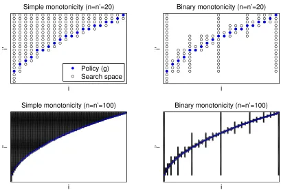
Figure 1 provides a graphical illustration of binary monotonicity and, for comparison, simple monotonicity. The blue dots represent the optimal policy (bn0pi/n0c in this case)
and the black empty circles represent, for a giveni, the search space when solving for g(i), i.e., the range ofi0 that might possibly be optimal. With simple monotonicity, the search for i >1 is restricted to{g(i−1), . . . , n0}. For binary monotonicity, the search is restricted to {g(i), . . . , g(i)}whereiandiare far apart for the first iterations but become close together rapidly (with the distance roughly halved at each iteration). For this example, the average search space for simple monotonicity, i.e. the average size of {g(i−1), . . . , n0}, is 8.7 when n = n0 = 20 and grows to 35.3 when n = n0 = 100. Since the search space for brute force would be be 20 and 100, respectively, this represents roughly a 60% improvement on brute force. In contrast, the average size of binary monotonicity’s search space is 6.2 when n=n0 = 20 (a 29% improvement on simple monotonicity) and 8.9 when n=n0 = 100 (a 75% improvement).
The remaining sections show that this example is typical. Specifically, in Section 3
we show that binary monotonicity always—i.e., for any monotone g—exhibits a very slow increase in search space as n increases. In contrast, simple monotonicity may not exhibit any reduction in search space (which is what happens when g(·) = 1). Then, in Section 4, we show that, for both the RBC andArellano(2008) models, simple monotonicity is about 60% faster than brute force. In contrast, binary monotonicity is much faster than simple monotonicity for small grids (e.g., six times faster whenn=n0 = 100) and increasingly so for larger grids (e.g., 27 times faster when n=n0 = 500).
2.4 Sufficient Conditions for Monotone Policies
i
i’
Binary monotonicity (n=n’=20)
i
i’
Simple monotonicity (n=n’=20)
Policy (g) Search space
i
i’
Binary monotonicity (n=n’=100)
i
i’
Simple monotonicity (n=n’=100)
Figure 1: A Graphical Illustration of Simple and Binary Monotonicity
Proposition 1. Let
V(b) = max
c≥0,b0∈Bu(c) +W(b
0) s.t. c=c(b, b0)
with W strictly increasing, u differentiable, strictly increasing, and strictly concave, and
c(b, b0) strictly increasing in b for every b0.
Defineδ(b, b02, b01) =c(b, b01)−c(b, b02) and suppose that forb02 > b01,δ is weakly decreasing in b. Then every optimal policy is weakly increasing (over the domain of b such that a feasible choice exists, {b| ∃b0 ∈ B s.t. c(b, b0)≥0}).
IfW is only weakly increasing but the other conditions are satisfied, then for each optimal policy that is not weakly increasing, there is another optimal policy that is.
Key to this result is that concavity and differentiability are only required for the period utility function,u, rather than the continuation utility W. Consequently, theW term can by the upper envelope of functions and exhibit non-concavities.
Lemma 1. Ifc(b, b0)can be written asc(b, b0) =f(b)+g(b0)for anyf andg, thenδ(b, b02, b01)
is weakly decreasing in b for b02 > b01.
Lemma 2. If c(b, b0) can be written as c(b, b0) = f(b) +g(b0) +m(b)n(b0) for any f and g
and for m and n increasing, thenδ(b, b02, b01) is weakly decreasing in b for b02> b01.
Many problems in economics meet these sufficient conditions, and we list several im-portant ones. In Aiyagari (1994), c(b, b0) = we+b(1 + r) −b0 where w and r are fac-tor prices and e is a household’s labor productivity, and Lemma 1 applies. In Chatter-jee et al. (2007), c(b, b0) = we+b−q(b0, e)b0, and Lemma 1 applies. In Arellano (2008), c(b, b0) = y+b−q(b0, y)b0, and Lemma 1 applies. In Hatchondo and Martinez (2009) and
Chatterjee and Eyigungor (2012), c(b, b0) =y+κb−q(b0, y)b0+ (1−κ)q(b0, y)b, and, since it can be shown that q is increasing inb0, Lemma 2applies.8
In some models, one might only be able to prove that W is weakly increasing. E.g., in the Arellano (2008) model, W(b0) = βP
y0πyy0max{Vd(y0), Vnd(b0, y0)} and there may be a range of b0 such that Vd is always greater than Vnd for all y0. While Proposition 1
guarantees restricting attention to monotone policies is without loss of generality, it may be desirable to ensure that all optimal policies are monotone. This can be accomplished fairly easily in theArellano(2008) model, and potentially in others, by a small transformation of the problem.9
3
Theoretical Analysis
In the preceding algorithm, we assume there is some method for solving
max
i0∈{a,...,a+γ−1}π(i, i
0
) (11)
for arbitrary a ≥ 1 and γ ≥ 1 (satisfying a+γ −1 ≤ n0). One possibility is brute force (checking every possible value), which requires γ evaluations of π(i,·). However, if π(i, i0) is known to be concave in i0, then Heer and Maußner (2005)’s binary concavity can find
8
Chatterjee and Eyigungor(2012) establish (1) thatq is monotone inb0 ifb0(b, y) is monotone inband (2) that, given a monotoneq,b0(b, y) is monotone.Hatchondo and Martinez(2009) has virtually the same setup asChatterjee and Eyigungor(2012) except that it uses a couponless bond.
9
SinceVndis strictly increasing inb0, points whereW is not strictly increasing inb0imply the probability of default is one, in which caseq(b0, y) = 0 for suchb0. It is well known thatb0= 0 is weakly better than such a point (since the continuation utility and consumption are both weakly higher). Consequently, the problem can be recast in a way that ensuresW is strictly increasing by redefiningW as
W(b0) =
βP
y0πyy0max{Vd(y0), Vnd(b0, y0)} ifq(b0, y)>0 b0+βP
y0πyy0max{Vd(y0), Vnd(b0, y0)} otherwise
the solution in no more than 2dlog2(γ)e −1 for γ ≥3 and γ for γ ≤2, which we prove in Lemma4in AppendixB. We allow for many such methods by characterizing the algorithm’s properties conditional on a monotonically increasingσ :Z++→Z+.
Because of the recursive nature of the algorithm, theπ evaluation bound for generalσis also naturally recursive. The following definition and Proposition 2provide such a bound.
Definition. For any σ : Z++ → Z+, define Mσ : {2,3, . . .} ×Z+ → Z+ recursively by Mσ(z, γ) = 0 if z= 2 or γ = 0 and
Mσ(z, γ) =σ(γ) + max γ0∈{1,...,γ}
n
Mσ(b
z
2c+ 1, γ
0) +M
σ(b
z
2c+ 1, γ−γ
0+ 1)o
for z >2 and γ >0.
Proposition 2. Let σ : Z++ → Z+ be an upper bound on the number of π evaluations required to solve (11). Then, the algorithm requires at most 2σ(n0) +Mσ(n, n0) evaluations
where n and n0 are from the problem stated in (1) for n≥2 and n0 ≥1.
Proposition 2 gives a fairly tight bound. However, it is also unwieldy because of the discrete nature of the problem. By bounding σ whose domain is Z++ with a ¯σ whose domain is [1,∞), a more convenient bound can be found. This bound is given in Lemma3.
Lemma 3. Suppose σ¯ : [1,∞) →R+ is either the identity map (¯σ(γ) =γ) or is a strictly
increasing, strictly concave, and differentiable function. If ¯σ(γ) ≥ σ(γ) for all γ ∈ Z++, then an upper bound on function evaluations is
3¯σ(n0) +
I−2
X
j=1
2jσ(2¯ −j(n0−1) + 1)
if I >2 where I =dlog2(n−1)e+ 1. An upper bound for I ≤2 is3¯σ(n0).
The main theoretical result of the paper is given in Proposition 3. It applies Lemma 3
with ¯σ bounds corresponding to brute force concavity and binary concavity.
Proposition 3. Suppose n≥4 and n0 ≥3. If brute force grid search is used, then binary monotonicity requires no more than (n0−1) log2(n−1) + 3n0 + 2n−4 evaluations of π. Consequently, fixingn=n0 the algorithm’s worst case behavior isO(nlog2n) with a hidden constant of one.
These worst-case bounds show binary monotonicity is very powerful, even without an assumption about concavity. The remainder of the paper assesses binary monotonicity’s performance in two economic models commonly employed in practice. As will be seen, binary monotonicity also does very well in the context of these models.
4
Comparison with Existing Grid Search Techniques
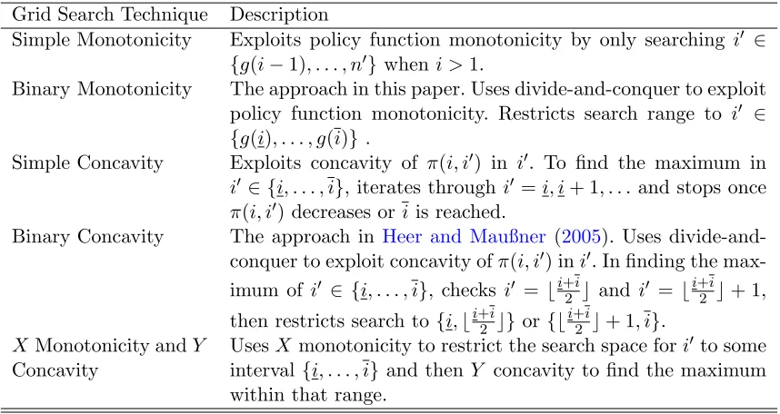
This section compares our method with existing grid search techniques. We do not conduct any error analysis, such as checking the Euler equation errors, since all the techniques deliver identical solutions. Table 1lists all techniques known to us (apart from brute force), along with brief descriptions of each. We break the analysis into two parts. First, we compare our method with existing techniques that do not assume concavity. For this, we use the
Arellano (2008) model. Second, we compare our method with existing techniques that do assume concavity. For this, we use the RBC model. Appendix Cgives the calibrations.
Grid Search Technique Description
Simple Monotonicity Exploits policy function monotonicity by only searching i0 ∈ {g(i−1), . . . , n0} wheni >1.
Binary Monotonicity The approach in this paper. Uses divide-and-conquer to exploit policy function monotonicity. Restricts search range to i0 ∈ {g(i), . . . , g(i)}.
Simple Concavity Exploits concavity of π(i, i0) in i0. To find the maximum in i0 ∈ {i, . . . , i}, iterates through i0 =i, i+ 1, . . . and stops once π(i, i0) decreases oriis reached.
Binary Concavity The approach in Heer and Maußner (2005). Uses divide-and-conquer to exploit concavity ofπ(i, i0) ini0. In finding the max-imum of i0 ∈ {i, . . . , i}, checks i0 = bi+2ic and i0 = bi+2ic+ 1, then restricts search to {i,bi+2ic} or{bi+2ic+ 1, i}.
XMonotonicity andY Concavity
UsesXmonotonicity to restrict the search space fori0 to some interval{i, . . . , i} and thenY concavity to find the maximum within that range.
Table 1: Description of Grid Search Techniques
4.1 Not Assuming Concavity
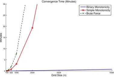
force. In contrast, binary monotonicity grows almost linearly. For a grid size of 100, all the methods solve the model in much less than a minute. This changes quickly with n. For a 1000 point grid, brute force takes about 8 minutes, simple monotonicity takes about half that, but binary monotonicity takes far less than a minute.
100 500 1000 2500 5000 10000
0 5 10 15 20 25 30
Convergence Time (Minutes)
Grid Size (n)
Minutes
Binary Monotonicity Simple Monotonicity Brute Force
Figure 2: Convergence Time For Methods Not Assuming Concavity
Run Time (Minutes) Evaluations/n Simple to Grid size (n) None∗ Simple∗ Binary∗ None∗ Simple∗ Binary∗ Binary Time
100 0.08∗ 0.03∗ 0.01∗ 100∗ 42∗ 5.5∗ 6.1
250 0.48∗ 0.20∗ 0.01∗ 250∗ 102∗ 6.1∗ 14.4 500 1.90∗ 0.78∗ 0.03∗ 500∗ 204∗ 6.5∗ 26.7 1000 7.71∗ 3.16∗ 0.06∗ 1000∗ 406∗ 7.0∗ 51.4 2500 47.7∗ 19.3∗ 0.17∗ 2500∗ 1013∗ 7.6∗ 116 5000 192∗ 78.6∗ 0.36∗ 5000∗ 2025∗ 8.0∗ 220 10000 769∗ 309∗ 0.75∗ 10000∗ 4050∗ 8.5∗ 409 25000 4814∗ 1914∗ 2.21∗ 25000∗ 10122∗ 9.1∗ 867 50000 19264∗ 7634∗ 4.60∗ 50000∗ 20243∗ 9.5∗ 1659 100000 77075∗ 30491∗ 8.91∗ 100000∗ 40484∗ 10.0∗ 3423 Note:∗ means the value is estimated via a fitted quadratic polynomial.
Table 2: Run Times and Evaluations for Methods Only Exploiting Monotonicity
4.2 Assuming Concavity
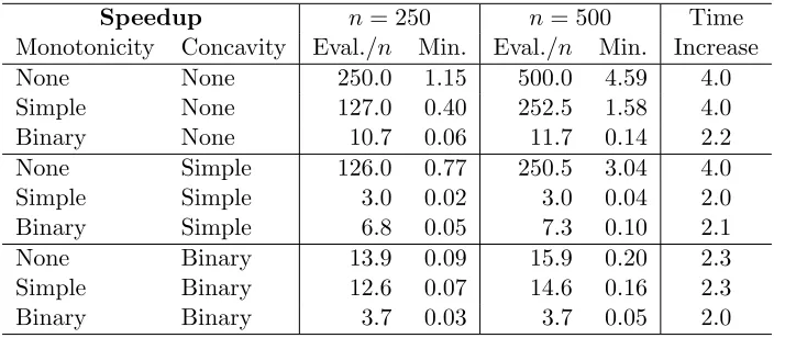
The previous section showed that binary monotonicity outperforms existing grid search methods that do not assume concavity. However, binary monotonicity can be combined with various concavity techniques to deliver potentially much faster performance. Table 3
examines the running times for all nine combinations of the monotonicity and concavity techniques. Since the Arellano (2008) model has a non-concave value function, the RBC model is used.
Speedup n= 250 n= 500 Time
Monotonicity Concavity Eval./n Min. Eval./n Min. Increase
None None 250.0 1.15 500.0 4.59 4.0
Simple None 127.0 0.40 252.5 1.58 4.0
Binary None 10.7 0.06 11.7 0.14 2.2
None Simple 126.0 0.77 250.5 3.04 4.0
Simple Simple 3.0 0.02 3.0 0.04 2.0
Binary Simple 6.8 0.05 7.3 0.10 2.1
None Binary 13.9 0.09 15.9 0.20 2.3
Simple Binary 12.6 0.07 14.6 0.16 2.3
Binary Binary 3.7 0.03 3.7 0.05 2.0
Table 3: Run Times and Evaluations for All Monotonicity and Concavity Speedups
concavity, exhibits a similar linear time increase but fares slightly worse in absolute terms. In particular, it requires on average 3.7 evaluations ofπ per state, a very small number, but not quite as small as the 3.0 required by simple concavity and simple monotonicity. All the other combinations are slower and exhibit superlinear time increases.
Although Table 3 only reports the performance for two grid sizes, it is representative. This can be seen in Figure3, which plots the average number ofπ evaluations required for four of the methods. Simple monotonicity with simple concavity and binary monotonicity with binary concavity both appear to beO(n) (with the latter guaranteed to be), but the hidden constant is smallest for the former. The other methods employing binary monotonic-ity grow atO(nlog2n), as predicted by the theory.
1000 10000 100000
2 4 6 8 10 12 14 16 18 20
Average # of Evaluations Divided by n
Grid Size (n)
Evaluations
Simple Mono, Simple Conc Binary Mono, No Conc Binary Mono, Simple Conc Binary Mono, Binary Conc
Figure 3: Empirical O(n) Behavior
Simple monotonicity paired with simple concavity is very effective because the policy function is nearly linear. In particular, the capital policy very nearly satisfiesg(i) =g(i−1)+ 1. In this case, simple monotonicity and simple concavity requires only threeπ evaluations to compute g(i) when g(i−1) is known: Evaluating π(i, g(i−1)), π(i, g(i−1) + 1), and π(i, g(i−1) + 2), the algorithm findsπ(i, g(i−1) + 1)≥π(i, g(i−1) + 2) and stops.
while binary monotonicity with binary concavity is not the fastest combination, it is still very fast. As Table3 shows, forn= 500 it is roughly 100 times faster than brute force and can solve a standard RBC model in just a few seconds.
5
Extensions
In this section, we consider continuous problems, portfolio choice, monotonicity in multiple state variables, and parallelization.
5.1 Continuous Problems
The algorithm has been described and analyzed for discrete states and choice sets, which allows for clean theoretical and empirical results. However, the logic readily extends to the continuous case. To be concrete, consider a monotone policy h that, for simplicity, maps the interval [x, x] into itself. By necessity, one would only be able to solve for the optimal policy at a finite number of points (one could then interpolate to obtain a value away from these points). So, let these points be given by {x1, x2, . . . , xn} with xi < xi+1. Defining
g(i) =h(xi), it is clear that g, defined fori= 1, . . . , n, is monotone.
The challenge then is in the search space, which is a continuous interval [x, x]. Here, if the objective function π(x, x0) is not single-peaked in x0, there is no completely reliable way of finding the maximum. One possibility is to perform a coarse grid search followed by a golden section search. Regardless of which method one chooses, one can exploit the monotonicity of g to narrow the search space. In particular, assuming that the policy has been found for some i and i, one can then solve for the policy at m := b(i+i)/2c by only searching in the interval [g(i), g(i)]. Having foundg(m), one could then use divide and conquer as in the discrete case.
An interesting extension of this approach would be an adaptive version of divide and conquer. In particular, one could choose a tolerance for the maximum allowable value of |h(xi)−h(xi+1)|. When this tolerance is exceeded, one could insert a grid point between
xi andxi+1, saym, and solve forh(m), which must be in the interval [h(xi), h(xi+1)]. This
process could be repeated as much as necessary and would eventually terminate if h is continuous. The computed policy’s error (measured in terms of the sup norm) would be less than the tolerance. To handle a discontinuoush, one could also require that|xi−xi+1|be
5.2 Portfolio Choice
In portfolio choice problems, it is very common that monotonicity does not obtain. For instance, Krusell and Smith (1997) consider a portfolio choice problem of a bond b0 and capital k0 taking as given some wealth ω. They show that the bond policy b0(ω) is not monotone in wealth (cf. Figure 3 in their paper). The reason is that at low levels of wealth, households would prefer to save in riskless bonds rather than risky capital, but prefer risky capital once they are sufficiently self-insured at higher wealth levels.
While the bond policy is not increasing in wealth, it is once conditioned on a choice of capital. To see this, consider a setup equivalent toKrusell and Smith (1997):
V(ω) = max
c≥0,b0∈B,k0∈Ku(c) +W(b
0, k0) s.t.c=c(ω, b0, k0) (12)
where W is strictly increasing in b0 (and k0) and where c(ω, b0, k0) = f(ω) +g(b0) +h(k0) for some g, h, and strictly increasing f. Here, b0(ω) and k0(ω) may not be monotonically increasing. However, after transforming this into a two-stage problem,
Vk(ω) = max
k0∈KV
b(ω, k0
) s.t.k0 has Vb(ω, k0) well-defined Vb(ω, k0) = max
c≥0,b0∈Bu(c) +W(b
0, k0) s.t.c=c(ω, b0, k0),
the policyb0b(ω, k0) associated withVb is monotonically increasing inω. This is because all the conditions of Proposition1and Lemma1are met.10This is despiteb0(ω) =b0b(ω, k0(ω)) not necessarily being increasing.
A natural question then is what sort of advantage binary monotonicity might bring to the problem (12). To answer this, let nω be the number of ω states and nk and nb be the cardinality of K and B, respectively. Then each Vb(·, k0) problem can be solved in no
more than 3nb+ 2nω+ log2(nω)nb evaluations of u(c) +W(b0, k0). Since there arenk of the Vb(·, k0) problems, the total required evaluations is 3nbnk+2nωnk+log2(nω)nbnk. Note that the cost increases linearly in nk since we are not exploiting (and generally cannot exploit)
monotonicity of b0 in k0. Nevertheless, fixing nb = nk = nω = n, binary monotonicity is O(log2(n)n2) whereas brute force is O(n3), a substantial improvement.
A special case of portfolio choice is when the assets are independent in terms of contin-uation utility, like in the problem
V(ω) = max
c≥0,a0z0∈A∀z0∈Z
u(c) + X
z0∈Z
Wz0(a0z0) s.t. c=f(ω) +
X
z0∈Z
gz0(a0z0), (13)
10
wheref is strictly increasing andWz0 is strictly increasing for eachz0. This type of problem occurs when the financial instruments are Arrow securities, or something akin to them (such as the defaultable Arrow securities inGordon,2015). In this case, one can transform this problem into #Z-stage problems each having only one control,a0z0, and only one state variable, cash at hand. The policy in each problem is then monotone and can be exploited using binary monotonicity. While we suspect the performance in this case is O(nlog2n) with a hidden constant of #Z, we are investigating this in ongoing research.
5.3 Monotonicity in Multiple State Variables
In this paper, the focus was on problems having one state i and one control i0 with the policy g(i) monotone increasing in i. In fact, there are numerous examples were there are two states i, j, one control i0, and g(i, j) is monotone in both arguments. For example, the problem
V(a, b) = max
c≥0,k0∈Ku(c) +W(k
0) s.t.c=f(a) +g(b) +h(k0) (14)
hask0(a, b) monotone increasing in bothaandbiff,g, andW are all strictly increasing.11In this case, it may be possible to use a divide-and-conquer algorithm to recursively subdivide the state spaceA × B and obtain significant speedup.
5.4 Parallelization
With the increasing number of cores available to programmers, parallelization is an im-portant issue. The binary monotonicity algorithm presented in Section 2.3 can be directly parallelized by doing an “n-section” rather than a bisection, distributing the divide and conquer step 2(c) to two threads, or parallelizing the maximization step. However, we sus-pect far greater speedup may be attained by distributing work over state variables not represented in the simple Π(i) = maxi0π(i, i0) formulation. For example, in mapping the
Arellano(2008) model to the form given in (1), we created separate problems for each value of outputy. Distributing distinctyvalues to threads is much coarser work than distributing work conditional on values ofy, and so we suspect it is likely to dominate in terms of speed for most applications.
11For a practical example, consider an Aiyagari (1994)-like model. Specifically, assume household have
earnings wεz—comprised of a factor price w, an i.i.d. shockε, and an AR1 shockz—and choose savings
b0 taking current savings b as given:c=wεz+b(1 +r)−b0 withr a factor price. Becauseε is i.i.d., the continuation utility could be written asW(b0, z) =βEV(b0, ε0, z0). Then it easy to show using Proposition
6
Conclusion
We have shown binary monotonicity is a powerful grid search technique. Without any as-sumption of concavity, the algorithm isO(nlog2n) for any monotone policy. Discrete choice models, where monotonicity obtains but concavity often does not, should substantially ben-efit from our approach. When paired with binary concavity, binary monotonicity is O(n) and so enables grid search to be used for very large grids. While simple monotonicity with simple concavity was empirically faster for the RBC model and calibration we used, bi-nary monotonicity with bibi-nary concavity offers guaranteed performance. We have outlined several promising extensions that are being analyzed in ongoing research.
References
S. R. Aiyagari. Uninsured idiosyncratic risk and aggregate savings. Quarterly Journal of Economics, 109(3):659–684, 1994.
C. Arellano. Default risk and income fluctuations in emerging economies. American Eco-nomic Review, 98(3):690–712, 2008.
C. Arellano, L. Maliar, S. Maliar, and V. Tsyrennikov. Envelope condition method with an application to default risk models. Mimeo, 2015.
S. B. Aruoba, J. Fern´andez-Villaverde, and J. F. Rubio-Ram´ırez. Comparing solution meth-ods for dynamic general equilibrium economies. Journal of Economic Dynamics and Control, 30(12):2477–2508, 2006.
C. D. Carroll. The method of endogenous gridpoints for solving dynamic stochastic opti-mization problems. Economic Letters, 91(3):312–320, 2006.
S. Chatterjee and B. Eyigungor. Maturity, indebtedness, and default risk. American Eco-nomic Review, 102(6):2674–2699, 2012.
S. Chatterjee, D. Corbae, M. Nakajima, and J.-V. R´ıos-Rull. A quantitative theory of unsecured consumer credit with risk of default. Econometrica, 75(6):1525–1589, 2007.
A. Clausen and C. Strub. A general and intuitive envelope theorem. Mimeo, 2013.
G. Fella. A generalized endogenous grid method for non-smooth and non-concave problems.
Review of Economic Dynamics, 17(2):329–344, 2014.
J. C. Hatchondo and L. Martinez. Long-duration bonds and sovereign defaults. Journal of International Economics, 79(1):117–125, 2009.
B. Heer and A. Maußner. Dynamic General Equilibrium Modeling: Computational Methods and Applications. Springer, Berlin, Germany, 2005.
P. Krusell and A. A. Smith, Jr. Income and wealth heterogeneity, portfolio choice, and equilibrium asset returns. Macroeconomic Dynamics, 1:387–422, 1997.
P. Krusell and A. A. Smith, Jr. Income and wealth heterogeneity in the macroeconomy.
Journal of Political Economy, 106(5):867–896, 1998.
G. Tauchen. Finite state Markov-chain approximations to univariate and vector autoregres-sions. Economics Letters, 20(2):177–181, 1986.
A
Algorithms
This appendix contains a non-recursive version of binary monotonicity, as well as our im-plementation of binary concavity.
A.1 A Non-Recursive Formulation of Binary Monotonicity
Rather than directly implementing binary monotonicity using recursion, it is computation-ally more efficient to eliminate the recursion. The following algorithm does this:
1. Initialization: Compute g(1) maximizing over {1, . . . , n0} and compute g(n) maxi-mizing over{g(1), . . . , n0}. Allocate an array of size (dlog2(n−1)e+ 1)×2 that will hold the list below. Fill the first row of the array with (l1, u1) wherel1 := 1,u1 :=n.
Define k:= 1.
2. Expand the list from krows to ˜k rows as follows:
l1 u1
.. . ... lk uk
lk+1 uk+1
lk+2 uk+2
.. . ... l˜k u˜k
:=
l1 u1
..
. ... lk uk
lk blk+2ukc
lk blk+u2k+1c
..
. ...
lk b lk+uk˜−1
stopping whenuk˜≤l˜k+ 1 (corresponding to step 2(a) in the algorithm). At this step,
k≥1 andg(lj) andg(uj) are known for allj≤k. Forj=k+ 1, . . . ,˜k, computeg(uj)
by maximizing over the interval g(lj−1), . . . , g(uj−1). Taking each row as specifying
an interval and subdividing it into two intervals, the following row gives the leftmost subinterval.
At this point,gis known for everylanduin the list. Moreover, the interval correspond-ing to ˜khas exactly two elements,lk˜ anduk˜, which implies the policy g(lk˜), . . . , g(u˜k)
is known.
Define k:= ˜k. Go to step 3.
3. If k = 1, STOP. If uk = uk−1, then eliminate the last row of the list by setting
k:=k−1 and repeat this step. Otherwise, go to the next step.
4. If here, then uk < uk−1. Set (lk, uk) := (uk, uk−1). This step corresponds to moving
to the right subinterval of the interval corresponding to k−1. Go to step 2.
To better understand the logic of the algorithm, consider how it works when n= 5. The list’s progression is traced out in (15). A box around numberimeans thatg(i) is solved for in that step. The initialization step solves for the left and right bound. Step 2 repeatedly partitions [1 5], which one should think of as {1, . . . ,5}, until it has only two elements, in this case corresponding to {1,2}. Each time it partitions, it solves for exactly one value of g, namely, the midpoint of the smallest current interval. So, for instance, when step 2 is first encountered, the list is just [1 5], and so the smallest interval is {1, . . . ,5}. It then solves for g(3) and makes the smallest interval {1,2,3}. It then bisects again, solving for g(2) and making the smallest interval {1,2}. Step 2 always moves “left” when it bisects. For instance, when it divides {1, . . . ,5}in half, it moves to{1,2,3}rather than {3,4,5}.
h
1 5
i
| {z }
Step 1 ⇒ 1 5 1 3 1 2
| {z }
Step 2 ⇒ 1 5 1 3 2 3
| {z }
Step 4 ⇒ " 1 5 1 3 #
| {z }
Step 3 ⇒ " 1 5 3 5 #
| {z }
Step 4 ⇒ 1 5 3 5 3 4
| {z }
Step 2 ⇒ 1 5 3 5 4 5
| {z }
Step 4
⇒h1 5
i
| {z }
Step 3
from left to right: Step 2 checks left subintervals, but when there are no left subintervals remaining, step 4 moves to the right.
Step 3 determines when it is time to move “up” and to the right. For instance, after the first time step 4 is encountered in (15), g is known for every value in {1, . . . ,3}, but not every value in{3, . . . ,5}. Step 3 signals it is time to move from {1, . . . ,3} to{3, . . . ,5} by deleting the fine partition{2,3}. Step 4, which always comes after step 3, then moves to the right by replacing [1 3] with [3 5]. When there are no more right partitions, the algorithm terminates.
A.2 Binary Concavity
Below is our implementation ofHeer and Maußner (2005)’s algorithm for solving
max
i0∈{a,...,b}π(i, i
0
).
Throughout, nrefers tob−a+ 1.
1. Initialization: If n= 1, compute the maximum, π(i, a), and STOP. Otherwise, set the flags 1a = 0 and 1b = 0. These flags indicate whether the value of π(i, a) and
π(i, b) are known, respectively.
2. Ifn > 2, go to 3. Otherwise,n= 2. Computeπ(i, a) if1a= 0 and compute π(i, b) if
1b = 0. The optimum is the best ofa, b.
3. If n > 3, go to 4. Otherwise, n = 3. If max{1a,1b} = 0, compute π(i, a) and set
1a= 1. Definem= a+2b, and compute π(i, m).
(a) If 1a = 1, check whetherπ(i, a) > π(i, m). If so, the maximum is a. Otherwise,
the maximum is eitherm orb; redefine a=m, set 1a= 1, and go to 2.
(b) If 1b = 1, check whether π(i, b) > π(i, m). If so, the maximum is b. Otherwise,
the maximum is eitheraorm; redefine b=m, set 1b = 1, and go to 2.
4. Here, n ≥ 4. Define m = ba+2bc and compute π(i, m) and π(i, m+ 1). If π(i, m) < π(i, m+ 1), a maximum is in{m+ 1, . . . , b}; redefinea=m+ 1, set1a= 1, and go to
2. Otherwise, a maximum is in{a, . . . , m}; redefine a=m, set1b = 1, and go to 2.12
B
Omitted Proofs and Lemmas
This section contains omitted proofs and lemmas. They are broken into three sections. Sec-tionB.1gives the proofs for the sufficient conditions for monotonicity. SectionB.2examines
12
the properties of the binary monotonicity algorithm and to a lesser extent the binary con-cavity algorithm. SectionB.3state in what sense (1) and (2) are equivalent and proves their equivalence.
B.1 Sufficient conditions
Proof of Proposition 1.
Proof. Consider the case ofW strictly increasing. Letb1 < b2and suppose, for contradiction,
that g1 :=g(b1) > g2 := g(b2). Define B(b) := {b0 ∈ B|c(b, b0) ≥ 0}, and note B is weakly
increasing since cis increasing inb.
First, suppose g2 ∈/ B(b1). Then c(b1, g2) < 0 ≤c(b1, g1) ⇒ c(b1, g2)−c(b1, g1) <0 or
δ(b1, g1, g2)<0. Then since g1 > g2, δ is weakly decreasing inb implying δ(b2, g1, g2)<0.
Then c(b2, g2) < c(b2, g1), and so u(c(b2, g2)) < u(c(b2, g1)). Because g2 < g1, W(g2) ≤
W(g1), which implies u(c(b2, g2)) +W(g2) < u(c(b2, g1)) +W(g1). This means g2 is not
optimal, which is a contradiction. Therefore,g2 must be in B(b1).
Because B is monotone increasing, g1 ∈ B(b2) since g1 ∈ B(b1). The optimality of g2
then implies
u(c(b2, g2)) +W(g2)≥u(c(b2, g1)) +W(g1) (16)
Also, since g2 ∈B(b1), the optimality ofg1 implies
u(c(b1, g1)) +W(g1)≥u(c(b1, g2)) +W(g2). (17)
Since g1 > g2, an implication of (16) is then that c(b2, g2) ≥ c(b2, g1) (since W(g1) ≥
W(g2)) with a strict inequality if W is strictly increasing. This implies δ(b2, g1, g2) =
c(b2, g2)−c(b2, g1) ≥ 0 (strict if W is strictly increasing). Also, since g1 > g2, δ(·, g1, g2)
is weakly decreasing. So, δ(b1, g1, g2) ≥δ(b2, g1, g2). Putting these together, δ(b1, g1, g2) ≥
δ(b2, g1, g2)>0 ifW is strictly increasing andδ(b1, g1, g2)≥δ(b2, g1, g2)≥0 ifW is weakly
increasing.
The two inequalities (16) and (17) together imply
u(c(b2, g2)) +W(g2)−u(c(b2, g1))−W(g1)≥0≥u(c(b1, g2)) +W(g2)−u(c(b1, g1))−W(g1)
and so imply
u(c(b2, g2))−u(c(b2, g1))≥u(c(b1, g2))−u(c(b1, g1)). (18)
Then becauseu is differentiable, (18) is equivalent to
Z c(b2,g2)−c(b2,g1) 0
u0(c(b2, g1) +x)dx≥
Z c(b1,g2)−c(b1,g1) 0
u0(c(b1, g1) +x)dx
or
Z δ(b2,g1,g2)
0
u0(c(b2, g1) +x)dx≥
Z δ(b1,g1,g2)
0
u0(c(b1, g1) +x)dx.
Since δ(b1, g1, g2)≥δ(b2, g1, g2),
Z δ(b2,g1,g2)
0
u0(c(b2, g1) +x)−u0(c(b1, g1) +x)
dx≥
Z δ(b1,g1,g2)
δ(b2,g1,g2)
u0(c(b1, g1) +x)dx
implying
Z δ(b2,g1,g2)
0
u0(c(b2, g1) +x)−u0(c(b1, g1) +x)
dx≥0. (19)
Now, since c is strictly increasing in b, c(b2, g1) > c(b1, g1). Hence, u0(c(b2, g1) +x) −
u0(c(b1, g1) +x)<0 for all positivex. IfW is strictly increasing, δ(b2, g1, g2)>0 and
0>
Z δ(b2,g1,g2)
0
u0(c(b2, g1) +x)−u0(c(b1, g1) +x)
dx≥0
gives a contradiction.
Now consider the case of W being only weakly increasing. Define G(b) as the argmax conditional on state b. Consider two points b2 > b1 such that an optimal policy is
non-monotone. That is, g1 ∈ G(b1), g2 ∈ G(b2), and g1 > g2. We will show in this case that
g1∈G(b2), and hence this non-monotonicity can be removed (i.e., without loss of generality,
the optimal policy can specifyg1 atb2 rather thang2). Since this can than be done at every
point of non-monotonicity, for every non-monotone optimal policy there is another optimal policy that is monotone.
With g1> g2, the arguments from above can be used to reestablish (19). (19) can only
hold if δ(b2, g1, g2) = 0, which implies c(b2, g2) = c(b2, g1). Using this and (16), W(g2) =
W(g1). Consequently,u(c(b2, g2)) +W(g2) =u(c(b2, g1)) +W(g1). Then, sinceg2 ∈G(b2),
g1 is also.
Proof. Let b2> b1 and b02 > b01. Then
δ(b2, b02, b
0
1)−δ(b1, b02, b
0
1) =c(b2, b01)−c(b2, b02)−c(b1, b01) +c(b1, b02)
=f(b2) +g(b01)−f(b2)−g(b02)−f(b1)−g(b01) +f(b1) +g(b02)
= 0
Proof of Lemma 2.
Proof. Let b2> b1 and b02 > b01. Then
δ(b2, b02, b
0
1)−δ(b1, b02, b
0
1) =c(b2, b01)−c(b2, b02)−c(b1, b01) +c(b1, b02)
=f(b2) +g(b01) +m(b2)n(b01)−f(b2)−g(b02)−m(b2)n(b02)
−f(b1)−g(b01)−m(b1)n(b10) +f(b1) +g(b02) +m(b1)n(b02)
=m(b2)(n(b01)−n(b
0
2))−m(b1)(n(b01)−n(b
0
2))
=−(m(b2)−m(b1))(n(b02)−n(b01))
≤0
B.2 Algorithm properties
As stated in the main text,σ is always assumed to be monotonically increasing.
Lemma 4. Consider the problem maxi0∈{a,...,a+n−1}π(i, i0) for any a and any i. For any n ∈ Z++, binary concavity requires no more 2dlog
2(n)e −1 evaluations if n ≥ 3 and no
more thann evaluations if n≤2.
Proof. We will show σ(n) = 2dlog2(n)e −1 for n≥3 and σ(n) = n forn≤2 is an upper bound on the number of evaluations the binary concavity requires. Forn= 1, the algorithm computes π(i, a) and stops, so one evaluation is required. This agrees with σ(1) = 1. For n = 2, two evaluations are required (π(i, a) and π(i, a+ 1)). This agrees with σ(2) = 2. Forn= 3,step 3 requiresπ(i, m) to be computed and may requireπ(i, a) to be computed. Then step 3(a) or step 3(b) either stop with no additional function evaluations or go to step 2 with max{1a,1b}= 1 where, in that case, at most one additional function evaluation
is required. Consequently, n= 3 requires at most three function evaluations, which agrees withσ(3) = 2dlog2(3)e −1 = 3. So, the statement of lemma holds for 1≤n≤3.
either{a, . . . , m}or{m+ 1, . . . , b} andπ(i, m) andπ(i, m+ 1) are computed in step 4, the
next step has max{1a,1b}= 1. Now, ifn= 4, the next step must be step 2, which requires
at most one additional evaluation (since max{1a,1b}= 1). Hence, the total evaluations are
less than or equal to 3 (two for step 4 and one for step 2). If n= 5, then the next step is either step 2, requiring one evaluation, or step 3, requiring two evaluations. So, the total evaluations are not more than four. Ifn= 6, the next step is step 3, and so four evaluations are required. Lastly, for n= 7, the next step is either step 3, requiring two evaluations, or step 4 (withn= 4), requiring at most three evaluations. So, the evaluations are weakly less than 5 = 2 + max{2,3}. Hence, for every n = 4,5,6, and 7, the required evaluations are less than 3,4,4,and 5, respectively. One can then verify that the evaluations are less than 2dlog2(n)e −1 for these values ofn.
Now, supposen≥4. We shall prove that the required number of evaluations is less than 2dlog2(n)e −1 (i.e., is less thanσ(n)). The proof is by induction. We have already verified the hypothesis holds forn∈ {4,5,6,7}, so consider somen≥8 and suppose the hypothesis holds for all m ∈ {4, . . . , n−1}. Let i be such that n ∈[2i+ 1,2i+1]. Then note that two things are true,dlog2(n)e=i+1 anddlog2(bn+12 c)e=i.13Sincen≥4, the algorithm is in (or proceeds to) step 4, which requires two evaluations, and then proceeds with a new interval to step 4 (again). Ifnis even, the new interval has sizen/2. Ifnis odd, the new interval either has a size of (n+ 1)/2 or (n−1)/2. So, ifnis even, no more than 2 +σ(n/2) evaluations are required; ifnis odd, no more than 2 + max{σ((n+ 1)/2), σ((n−1)/2)}= 2 +σ((n+ 1)/2) evaluations are required. The even and odd case can then be handled simultaneously with the bound 2 +σ(bn+12 c). Manipulating this expression using the previous observation that dlog2(n)e=i+ 1 and dlog2(bn+12 c)e=i,
2 +σ(bn+ 1
2 c) = 2 + 2dlog2b n+ 1
2 ce −1 = 2 + 2i−1
= 2(i+ 1)−1
= 2dlog2(n)e −1.
Hence, the proof by induction is complete.
Lemma 5. For any σ, Mσ(z, γ) is weakly increasing in z and γ.
Proof. Fix a σ and suppress dependence on it. First, we will show M(z, γ) is weakly
in-13The proof is the following. Both dlog
2(·)e and dlog2(b·c)e are weakly increasing functions. So n ∈
[2i+ 1,2i+1] implies dlog2(n)e ∈ [dlog2(2 i
+ 1)e,dlog2(2 i+1
)e] = [i+ 1, i+ 1]. Likewise, dlog2(bn+12 c)e ∈
[dlog2(b2i+1+1
2 c)e,dlog2(b 2i+1+1
creasing in γ for every z. The proof is by induction. For z = 2, M(2,·) = 0. For z = 3, M(3, γ) = σ(γ) which is weakly increasing in γ. Now consider some z > 3 and suppose M(y,·) is weakly increasing for all y≤z−1. Forγ2 > γ1,
M(z, γ1) =σ(γ1) + max
γ0∈{1,...,γ
1}
n
M(bz
2c+ 1, γ
0
) +M(bz
2c+ 1, γ1−γ
0
+ 1)
o
≤σ(γ2) + max
γ0∈{1,...,γ
2}
n
M(bz
2c+ 1, γ
0
) +M(bz
2c+ 1, γ1−γ
0
+ 1)
o
≤σ(γ2) + max
γ0∈{1,...,γ
2}
n
M(bz
2c+ 1, γ
0) +M(bz
2c+ 1, γ2−γ
0+ 1)o
=M(z, γ2)
where the second inequality is justified by the induction hypothesis givingM(bz2c+ 1,·) as an increasing function (notebz
2c+ 1≤z−1 for allz >3).
Now we will show M(z, γ) is increasing in z for every γ. The proof is by induction. First, note that M(2, γ) = 0 ≤σ(γ) = M(3, γ) for all γ > 0 and M(2, γ) = 0 = M(3, γ) forγ = 0. Now, consider somek >3 and suppose that for any z1, z2 ≤k−1 with z1 ≤z2
thatM(z1, γ)≤M(z2, γ) for allγ. The goal is to show that for any z1, z2≤k withz1 ≤z2
thatM(z1, γ)≤M(z2, γ) for allγ. So, consider suchz1, z2 ≤k withz1 ≤z2. Ifγ = 0, then
M(z1, γ) = 0 =M(z2, γ), so take γ >0. Then
M(z1, γ) =σ(γ) + max
γ0∈{1,...,γ}
n
M(bz1
2c+ 1, γ
0
) +M(bz1
2c+ 1, γ−γ
0
+ 1)
o
≤σ(γ) + max
γ0∈{1,...,γ}
n
M(bz2
2c+ 1, γ
0
) +M(bz2
2c+ 1, γ−γ
0
+ 1)
o
=M(z2, γ).
The inequality obtains sincebzi
2c+ 1≤k−1 for alli(which is true since even ifzi =k, one
hasbk/2c+1≤k−1 by virtue ofk >3). So, the induction hypothesis givesM(bz1
2c+1,·)≤
M(bz2
2c+ 1,·), and the proof by induction is complete.
Proof of Proposition 2.
Proof. Since g is the policy function associated with (1), g :{1, . . . , n} → {1, . . . , n0}. By monotonicity,g is weakly increasing. DefineN :{1, . . . , n}2→
Z+ by
N(a, b) =M(b−a+ 1, g(b)−g(a) + 1)
define a sequence of setsIk fork= 1, . . . , n−1 by
Ik:={(i, i)|i=i+kand i, i∈ {1, . . . , n}}.
Note that for any k ∈ {1, . . . , n−1}, Ik is nonempty and N(a, b) is well-defined for any (a, b)∈ Ik.
We shall now prove that for anyk∈ {1, . . . , n−1}, (i, i)∈ IkimpliesN(i, i) is an upper
bound on the number of evaluations ofπ required by the algorithm in order to compute the optimal policy for all i∈ {i, . . . , i} when g(i) and g(i) are known. If true, then beginning at step 2 in the algorithm (which assumes g(i) andg(i) are known) with (i, i)∈ Ik,N(i, i)
is an upper bound on the number of π evaluations.
The argument is by induction. First, consider k= 1. For any (a, b)∈ I1, the algorithm
terminates at step 2(a). Consequently, the number of requiredπ evaluations is zero, which is the same as N(a, b) = M(b−a+ 1, g(b)−g(a) + 1) =M(2, g(b)−g(a) + 1) = 0 (recall M(2,·) = 0).
Now, consider some k∈ {2, . . . , n−1} and suppose the induction hypothesis holds for all j in 1, . . . , k−1. That is, assume for all j in 1, . . . , k−1 that (i, i) ∈ Ij implies N(i, i) is an upper bound on the number of requiredπ evaluations wheng(i) andg(i) are known. We shall show it holds fork as well.
Consider any (i, i)∈ Ikwithg(i) andg(i) are known. Sincei > i+ 1, the algorithm does not terminate at step 2(a). In step 2(b), to compute g(m) (where m := bi+2ic), one must find the maximum within the rangeg(i), . . . , g(i), which requires at mostσ(g(i)−g(i) + 1) evaluations of π. In step 2(c), the space is then divided into{i, . . . , m} and{m, . . . , i}.
than
σ(γ) +M(m−i+ 1, g(m)−g(i) + 1) +M(i−m+ 1, g(i)−g(m) + 1)
=σ(γ) +M(i+i
2 −i+ 1, γ
0) +M(i−i+i
2 + 1, g(i)−g(m) + 1) =σ(γ) +M(i−i
2 + 1, γ
0
) +M(i−i
2 + 1, g(i)−g(m) +γ
0−
γ0+ 1)
=σ(γ) +M(i−i 2 + 1, γ
0) +M(i−i
2 + 1, g(i)−g(m) +g(m)−g(i) + 1−γ
0+ 1)
=σ(γ) +M(i−i 2 + 1, γ
0) +M(i−i
2 + 1, γ−γ
0+ 1).
By virtue of monotonicity, g(m) ∈ {g(i), . . . , g(i)} and sog(m)−g(i) + 1 ∈ {1, . . . , g(i)− g(i) + 1} or equivalentlyγ0 ∈ {1, . . . , γ}.Consequently, the number of function evaluations is not greater than
σ(γ) + max
γ0∈{1,...,γ}
M
i−i 2 + 1, γ
0
+M
i−i
2 + 1, γ−γ
0+ 1
.
The case ofkodd is very similar, but the divide-and-conquer algorithm splits the space unequally. If k is odd, then m equals i+2i−1. In this case (i, m) ∈ I(k−1)/2 and (m, i) ∈ I(k−1)/2+1.14 Consequently, computing the policy for i, . . . , i takes no more than σ(g(i)−
g(i)−1) +N(i, m) +N(m, i) maximization steps. Definingγ andγ0 the same as before and using the definition ofm and N, we have the the required maximization steps is less than
σ(γ) +M(m−i+ 1, γ0) +M(i−m+ 1, γ−γ0+ 1)
=σ(γ) +M(i+i−1
2 −i+ 1, γ
0) +M(i−i+i−1
2 + 1, γ−γ
0+ 1)
=σ(γ) +M
i−i+ 1 2 , γ
0
+M
i−i+ 1
2 + 1, γ−γ
0
+ 1
.
Because M is increasing in the first argument, this is less than
σ(γ) + max
γ0∈{1,...,γ}
M
i−i+ 1 2 + 1, γ
0
+M
i−i+ 1
2 + 1, γ−γ
0
+ 1
.
Combining the bounds for keven and odd, the required number ofπ evaluations is less
14
To see this, note that (i, i)∈ Ikimpliesk=i−i. To have, (i, m)∈ I(k−1)/2, it must be thatm=i+k−21.
This holds:i+k−1
2 =i+
i−i−1
2 =i+
i+i−1−i−i
2 =i+m+
−2i
2 =m. Similarly, to have (m, i)∈ I(k−1)/2+1,
than
σ(γ) + max
γ0∈{1,...,γ}
M
i−i+ 1 2
+ 1, γ0
+M
i−i+ 1 2
+ 1, γ−γ0+ 1
(*)
because if k is even, then bi−i2+1c = i−2i. Consequently, (*) gives an upper bound for any (i, i)∈ Ik fork≥1 wheng(i) andg(i) are known. IfN(i, i) is less than this, then the proof by induction is complete.
Since N(i, i) is defined asM(i−i+ 1, g(i)−g(i) + 1), using the definitions ofN andM shows
N(i, i) =M(i−i+ 1, g(i)−g(i) + 1) =M(i−i+ 1, γ)
=σ(γ) + max
γ0∈{1,...,γ}
M(bi−i+ 1
2 c+ 1, γ
0
) +M(bi−i+ 1
2 c+ 1, γ−γ
0
+ 1)
.
Consequently,N(i, i) exactly equals the value in (*), and the proof by induction is complete. Step 1 of the algorithm requires at most 2σ(n0) evaluations to computeg(1) and g(n). Ifn= 2, step 2 is never reached. SinceM(n, n0) = 0 in this case, 2σ(n0) +M(n, n0) provides an upper bound. Ifn > 2, then since (1, n)∈ In−1 and g(1) andg(n) known, onlyN(1, n)
additional evaluations are required. Therefore, to compute for each i∈ {1, . . . , n}, no more than 2σ(n0) +N(1, n) = 2σ(n0) +M(n, g(n)−g(1) + 1) function evaluations are needed. Lemma (5) then gives that this is less than 2σ(n0) + M(n, n0) since g(n) −g(1) + 1 ≤ n0−1 + 1 =n0.
Lemma 6. Define a sequence {mi}∞i=1 by m1 = 2 and mi = 2mi−1 −1 for i ≥ 2. Then
mi = 2i−1+ 1 and log2(mi−1) =i−1 for alli≥1.
Proof. The proof of mi = 2i−1+ 1 for all i≥1 is by induction. For i= 1,m1 is defined as
2, which equals 21−1+ 1. For i >1, suppose it holds fori−1. Then
mi = 2mi−1−1
= 2[2i−2+ 1]−1 = 2i−1+ 1.
Lemma 7. Consider any z ≥ 2. Then there exists a unique sequence {ni}Ii=1 such that
Proof. The proof that a unique sequence exists is by construction. Let z ≥ 2 be fixed. Define an infinite sequence {zi}∞i=1 recursively as follows: Define zi = Ti(z) for all i ≥ 1
withT1(z) :=z and Ti+1(z) =bTi2(z)c+ 1. We now establish all of the following:Ti(z)≥2,
Ti(z) ≥Ti+1(z), and Ti(z) > Ti+1(z) whenever Ti(z) > 2. As an immediate consequence,
for any z ≥ 2, there exists a unique I(z) ≥ 1 such that TI(z) = 2 and, for all i < I(z),
Ti(z)>2. We also show for later use thatTi(z) is weakly increasing inzfor every i.
To show Ti(z) ≥ 2, the proof is by induction. We have T1(z) = z and z ≥ 2. Now,
consider somei >1 and suppose it holds fori−1. ThenTi(z) =bTi−21(z)c+ 1≥ b22c+ 1 = 2.
To show Ti(z) > Ti+1(z) whenever Ti(z) > 2, consider two cases. First, considerTi(z)
even. Then Ti+1(z) =bTi2(z)c+ 1 = Ti2(z) + 1 and so Ti+1(z) < Ti(z) as long as Ti(z) >2.
Second, considerTi(z) odd. ThenTi+1(z) =bTi2(z)c+ 1 = Ti(z2)−1+ 1 and soTi+1(z)< Ti(z)
as long as Ti(z)>1.
To show that Ti(z) ≥ Ti+1(z), all we need to show now is that Ti+1(z) = 2 when
Ti(z) = 2 (since the inequality is strict if Ti(z) >2 and Ti(z) ≥2 for all i). If Ti(z) = 2,
thenTi+1(z) =b22c+ 1 = 2.
To establish that Ti(z) is weakly increasing in z for every i, the proof is by induction.
For a ≤ b, T1(a) = a ≤ b = T1(b). Now consider some i > 1 and suppose the induction
hypothesis holds fori−1. Then Ti(a) =bTi−1(a)/2c+ 1≤ bTi−1(b)/2c+ 1 =Ti(b).
The sequence {nj}Ij(=1z) defined bynj =TI(z)−j+1(z)—i.e., an inverted version of the
se-quence{Ti(z)}Ii=1(z)—satisfiesnI(z)=T1(z) =z,n1(z) =TI(z)= 2, andni−1=TI(z)−(i−1)+1=
bTI(z)−(i−1)
2 c+ 1 =b
ni
2 c+ 1. Also, by the definition ofI(z),Ti(z)>2 for any i > I(z). So,
if we can show thatI(z) =dlog2(z−1)e+ 1, the proof is complete.
The proof of I(z) = dlog2(z−1)e+ 1 is as follows. Note that for z = 2, the sequence {zi} is simply zi = 2 for all i which implies I(2) = 1. Since dlog2(2−1)e+ 1 = 1, the
relationship holds for z = 2. So, now consider z > 2. The proof proceeds in the following steps. First, for the special {mi} sequence defined in Lemma 6, we show Tj(mi) =mi+1−j
for anyi≥1 and anyj≤i. Second, we use this to show thatI(mi) =ifor alli≥1. Third,
we show thatz∈(mi−1, mi] implies I(z) =iby showingI(mi−1)< I(z)≤I(mi). Fourth,
we show that the isuch that z ∈(mi−1, mi] is given bydlog2(z−1)e+ 1. This then gives
I(z) =dlog2(z−1)e+ 1 sinceI(z) =I(mi) =i=dlog2(z−1)e+ 1.
First, we showTj(mi) =mi+1−j for anyi≥1 and anyj≤i. Fix somei≥1. The proof
and suppose the induction hypothesis holds for j−1. Then
Tj(mi) =b
Tj−1(mi)
2 c+ 1
=bmi+1−(j−1) 2 c+ 1 =bmi+2−j
2 c+ 1
=b2mi+1−j−1 2 c+ 1
=mi+1−j+b−
1 2c+ 1 =mi+1−j−1 + 1
=mi+1−j,
which proves Tj(mi) =mi+1−j forj≤i. The fourth equality follows from the definition of
{mi}in Lemma 6.
Second, we showI(mi) =ifor alli≥1. Fix anyi≥1. We just showedTj(mi) =mi+1−j.
Hence,Ti(mi) =m1 = 2 and Ti−1(mi) =m2 = 3. Consequently, the definition of I—which
for a givenzis defined as the smallesti≥1 such thatTi(z) = 2—givesI(mi) =i(recallTj
is decreasing in j).
Third, we show that z ∈ (mi−1, mi] implies I(z) = i by showing I(mi−1) < I(z) ≤
I(mi). Note that, since z > 2 (having taken care of the z = 2 case already), there is
some i ≥ 2 such that z ∈ (mi−1, mi] (since m1 = 2). To see I(z) ≤ I(mi), suppose not,
that I(z) > I(mi). But then 2 = TI(z)(z) < TI(mi)(z) ≤ TI(mi)(mi) = 2, which is a
contradiction.15 Therefore,I(z)≤I(mi).
To see I(mi−1)< I(z), we begin by showingTj(mi−1)< Tj(mi−1+ε) for anyε >0 and
any j ≤i−1. Since Tj(mi−1) = mi−j, it is equivalent to show thatmi−j < Tj(mi−1+ε),
which we show by induction. Clearly, forj = 1, we havemi−1 < mi−1+ε=T1(mi−1+ε).
Now considerj >1 and suppose it is true forj−1. Then
Tj(mi−1+ε) =b
Tj−1(mi−1+ε)
2 c+ 1
=bTj−1(mi−1+ε)−mi−j+1+mi−j+1
2 c+ 1
=bTj−1(mi−1+ε)−mi−j+1+ 2mi−j−1
2 c+ 1
=bTj−1(mi−1+ε)−mi−j+1−1
2 c+mi−j+ 1
Now, since the induction hypothesis of Tj−1(mi−1+ε) > mi−j+1 gives Tj−1(mi−1+ε)− 15The second inequality uses thatT
mi−j+1−1≥0, one has
Tj(mi−1+ε)≥ b
0
2c+mi−j+ 1 =mi−j+ 1
> mi−j.
Hence the proof by induction is complete.
Now, having established Tj(mi−1) < Tj(mi−1 +ε) for any ε > 0 and any j ≤ i−1,
we show I(mi−1) < I(z). Suppose not, that I(mi−1) ≥I(z). Then since z > mi−1, taking
ε=z−mi−1we have 2 =TI(mi−1)(mi−1)< TI(mi−1)(mi−1+ε) =TI(mi−1)(z)≤TI(z)(z) = 2, which is a contradiction.
Lastly, we now show that the i such that z ∈(mi−1, mi] is given by dlog2(z−1)e+ 1.
That this holds can be seen as follows. Note that z∈(mi−1, mi] implies log2(z−1) + 1∈
(log2(mi−1 −1) + 1,log2(mi −1) + 1]. Then, since log2(mj −1) + 1 = j for all j ≥ 1
(Lemma 6), we have log2(z−1) + 1 ∈ (i−1, i]. Then, by the definition of d·e, one has dlog2(z−1) + 1e=i, which of course is equivalent todlog2(z−1)e+ 1 =i.
We established the i such that z∈(mi−1, mi] is i=dlog2(z−1)e+ 1. Also we showed
i−1 =I(mi−1)< I(z) ≤I(mi) =i. HenceI(z) = dlog2(z−1)e+ 1, which completes the
proof.
Proof of Lemma 3.
Proof. In keeping with the notation of the other proofs, letzandγ correspond to nandn0, respectively. Fix some arbitraryz≥2. By Lemma7, there is a strictly monotone increasing sequence{zi}Ii=1 withzI =z,zi =bzi2+1c+ 1 fori < I, and withI =dlog2(z−1)e+ 1 (and
having z1 = 2).
For i >1 and any γ ≥1, define
W(zi, γ) := max
γ0∈{1,...,γ}M(zi−1, γ
0) +M(z
i−1, γ−γ0+ 1).
Fori= 1, defineW(zi,·) = 0. The definition ofM givesM(zi, γ) =σ(γ) +W(zi, γ) for any
i >1 with M(z1,·) = 0. Note thatW(z2, γ) =W(z1, γ) = 0.
Define ¯W—which we will demonstrate is an upper bound and continuous version of W—as
¯
W(zi, γ) := ¯σ∗(γ) + max γ0∈[1,γ]
¯