Attacking Data Transforming Learners at Training Time

The Thirty-Third AAAI Conference on Artificial Intelligence (AAAI-19)

Attacking Data Transforming Learners at Training Time

Scott Alfeld,

_{Ara Vartanian,}

_{Lucas Newman-Johnson,}

_{Benjamin I.P. Rubinstein}

1_{Department of Computer Science, Amherst College}

2_{Department of Computer Sciences, University of Wisconsin – Madison} 3_{School of Computing and Information Systems, University of Melbourne}

1_{{salfeld, lnewmanjohnson18}@amherst.edu} 2_{[email protected]}

3_{[email protected]}

Abstract

While machine learning systems are known to be vulnera-ble to data-manipulation attacks at both training and deploy-ment time, little is known about how to adapt attacks when the defender transforms data prior to model estimation. We consider the setting where the defender Bob first transforms the data then learns a model from the result; Alice, the at-tacker, perturbs Bob’s input dataprior to him transforming it. We develop a general-purpose “plug and play” framework for gradient-based attacks based on matrix differentials, focus-ing on ordinary least-squares linear regression. This allows learning algorithms and data transformations to be paired and composed arbitrarily: attacks can be adapted through the use of the chain rule—analogous to backpropagation on neural network parameters—to compositional learning maps. Best-response attacks can be computed through matrix multiplica-tions from a library of attack matrices for transformamultiplica-tions and learners. Our treatment of linear regression extends state-of-the-art attacks at training time, by permitting the attacker to affect both features and targets optimally and simultaneously. We explore several transformations broadly used across ma-chine learning with a driving motivation for our work being autogressive modeling. There, Bob transforms a univariate time series into a matrix of observations and vector of target values which can then be fed into standard learners. Under this learning reduction, a perturbation from Alice to a single value of the time series affects features of several data points along with target values.

Introduction

While outside the traditional focus of security, attacks on machine learning systems are inevitable: the very adaptabil-ity that learners deliver to valuable applications and indus-tries is also an attack surface to be exploited. A key security goal in adversarial machine learning research is model in-tegrity/availability (Barreno et al. 2006) or prediction cor-rectness more broadly. There, a defender Bob wishes to learn and then deploy a model after the adversary Alice has perturbed train or test data. While numerous positive results demonstrate the potential power Alice might wield in lab settings (Rubinstein et al. 2009; Biggio et al. 2013; Copyright c2019, Association for the Advancement of Artificial Intelligence (www.aaai.org). All rights reserved.

Szegedy et al. 2013), little is known about something as prevalent to practical scenarios as feature transformation and its effects on optimal attack strategies (Huang et al. 2011). This paper delivers a systematic treatment of opti-mal best-response attacks against a defender employing data pre-processing.

A common approach to computing data manipulation at-tacks is with a so-called gradient-based attack (Biggio et al. 2013), where Alice performs gradient-descent on her loss function to optimize her data perturbation. To compute the gradient we employ the theory of matrix differential calculus (MDC) (Magnus and Neudecker 1988). Manipulating dif-ferentials is more hospitable to compact calculation, though from a theoretical point of view the concepts of (matrix) dif-ferentials and (matrix) derivatives are equivalent. Through the chain rule, one can compute the gradient of Alice’s loss for any transform-learner combination via matrix (or tensor) multiplication. One need only compute the (matrix) deriva-tive of the learner and the derivaderiva-tive of the transform, sepa-rately. In this way, MDC yields a “plug and play” framework for generating adversarial perturbations.

A consequence is that much prior work — which focuses on settings where Alice directly affects the features or target values fed into the learner — can be leveraged to compute attacks against defenders which first transform the data. We illustrate this phenomenon by computing the derivative of ordinary least squares (OLS) regressionfor arbitrary addi-tive perturbationsand three different transforms within the MDC framework. We further demonstrate the flexibility of our framework by discussing the case when Bob performs a series of transforms prior to learning. Where prior work has often considered an attacker bound to specific types of alterations (e.g., affecting only target values or a single data point), we allow for an attacker to simultaneously alter both features and target values1. It is through algebraic manipula-tions of matrix differentials that we are able to compute the derivative of Alice’s loss.

A driving motivation for our work is autoregressive (AR) modeling. Here one models a value of a time series as some

1

function of the priordvalues of the same time series2. For example, suppose Alice and Bob are negotiating Bob’s pur-chase of Alice’s company. Bob might take the company’s historical quarterly profits as a time series and forecast fu-ture profits. So as to get as high a price as possible, Alice wants Bob to learn a model which forecasts high profits. She might “cook the books” and manipulate her company’s past profit numbers to trick Bob into learning such a model. Note that she may perform her manipulation in a legal way, by e.g., channel stuffing or earnings manipulation.

For example, Alice might reschedule sales so as to shift profits from one quarter to the following (or prior) quarter. Or she might move her costs (e.g., by changing the tim-ing of large purchases) to quarters showtim-ing poor perfor-mance. Her hope is then that that later quarters show an improvement/recovery, which Bob may see as positive mo-mentum. Prior work (Alfeld, Zhu, and Barford 2016) has examined deployment-time attacks against a fixed (autore-gressive) model. By contrast, we compute a training time attack.

There is strong real-world motivation to study attacks against autoregressive learners due to their use in e.g., the fi-nancial sector. In addition, such models demonstrate intrigu-ing behavior. To learn an autoregressive model, a learner can transform the time series into a collection of (feature, target) pairs which are then fed into an off-the-shelf ma-chine learning algorithm (Bontempi, Taieb, and Le Borgne 2012). This transformation from time series to features and targets causes single values (e.g., Alice’s profits for a par-ticular quarter) to be both features and a target value. For example, suppose Bob models the profits of a quarter as some function f of the previous two quarters from a se-ries of examples of the formQi = f(Qi−1, Qi−2).

Alter-ing Q3’s value will simultaneously affect three examples: Q3=f(Q2, Q1), Q4=f(Q3, Q2), Q5=f(Q4, Q3). This

fact that the attacker affects both features and target values distinguishes a contribution of our work from prior works in which the attacker affects only features (Jagielski et al. 2018) or only target values (Mei and Zhu 2015).

Forming a collection of (features, target) pairs from a time series is only one example of a data transformation step. Of-ten data is e.g., centered, normalized, standardized, etc. prior to learning and if Alice performs her data manipulation at-tack prior to this transformation, she must account for it in selecting her attack. We argue that a realistic model of an attacker is one where she affects data prior to the transfor-mation (which is, after all, performed by Bob).

This paper is organized as follows. First, we mathemat-ically define the agents Alice and Bob in terms of their knowledge and goals. We then calculate the derivative of Alice’s loss for OLS regression and a range of common data transformations. To empirically investigate the connection between Alice’s capability and her effectiveness as an at-tacker, we perform experiments on synthetic data. We then discuss the most closely related prior work and conclude.

2

dis known as theorderordegreeof the autoregressive model.

Problem Setup

We denote vectors by lower case bold characters (e.g.,vvv, θθθ) and matrices by upper case bold characters (e.g.,DDD, HHH). We denote the i-th element of a vector as the unbolded letter with a subscript (e.g., vi). We denote individual elements

of a matrix with brackets, using colons to denote an entire row, column (e.g.,XXX[:,1]denotes the first column of X). We denote the n×nidentity matrix as IIIn, and the

Kro-necker product by ⊗. Given a matrixAAA ∈ _Rm×n _we

de-note the mn×1 vector formed by stacking AAA’s columns asVec(AAA). We denote themn×mncommutator matrix as

K K

K(m,n)whereKKK(m,n)Vec(AAA) =Vec(AAA>) ∀AAA∈Rm×n. For matricesMMM ∈_Ra×b_{, andNNN ∈}

Rc×d, we define the derivative ofMMM with respect toNNN using the “Good Nota-tion” of Magnus and Neudecker (1988):

∇NNNMMM =

dVec(MMM) dVec(NNN)> ∈R

ab×cd

(1)

The i-th column of ∇NNNMMM (which is anab×1 vector) is

_dVec(MMM) dVec(NNN)i

>

. Note that this has the effect that whenMMM is a column vector andNNN is a scalar (represented as a1×1 matrix), then the gradient is a row vector.

Agent Definitions

We consider two agents: Alice the attacker and Bob the de-fender. Alice seeks to manipulate the model that Bob learns by exercising her limited capability to perturb his input data. Bob is oblivious to Alice and dutifully performs a transfor-mation on his input data followed by a machine learning algorithm to obtain a model. We model Alice as knowing both the transformation procedure and learning algorithm Bob uses. In what follows we define the specifics of the two players.

Bob the Defender After receiving data (potentially

per-turbed by the attacker Alice), Bob performs a two-step pro-cess. While typically the data that Bob receives will be in the form of a matrix of features and a vector of target values, this is not always the case. To remain general and have clean notation for our later examples, we simply say there aren

scalar values as input data. Bob first performs a transforma-tionT : Rn →R(p×d)×Rpto obtain a feature matrixXXX and vector3of target valuesyyy. We denote the matrix[yyy|XXX] asDDD. As a second step, Bob feedsXXX andyyyinto some fixed-length-vector learning algorithm. Specifically, Bob selects a modelθθθ∗from his hypothesis spaceΘwhich minimizes his loss`Bon the training data:

θθθ∗= argmin

θ θ θ∈Θ

`B(vvv;θθθ) (2)

For simplicity we assume a unique minimizer.

Alice the Attacker Alice can perturb the data that Bob

receives (before he performs his transformation on it). Her goal is to pull Bob’s learned model toward her specific target

θ θ

θtarget_{, captured by her loss function`}

A. For example, Alice

3

may have a target model which forecasts a particular pattern (e.g., a sharp increase in company profits) on some specific input (e.g., upcoming profit reports). Alice selects a vector

δδδ∈Rnas additive noise: Bob will observevvv+δδδ, then learn a model onT(vvv +δδδ). We assume a powerful attacker in terms of knowledge, but bounded in ability. Namely, Alice knowsvvv and Bob’sT and learner mappings. However, Al-ice is constrained to select her attack from some setC. This yields Alice’s bi-level optimization problem:

δδδ∗= argmin

δ δ δ

`A(θθθ∗) (3)

s.t.δδδ∈ C θ

θθ∗= argmin

θθθ∈Θ

`B(vvv+δδδ;θθθ)

Alice solves this problem using the common technique of projected gradient descent. Beginning with small random initialδδδ(0), she iteratively updates:

δδδ(t+1)=Proj_δδδ

δδδ(t)−η∇δδδ`A

θ θθ(t)

> (4)

θ θ

θ(t+1)= argmin

θ θθ∈Θ

`B

v v

v+δδδ(t+t);θθθ (5)

whereηdenotes her chosen step size and the functionProj

projects its argument to the nearest4_withinC:

Proj(δδδ0) = argmin

δ δδ

kδδδ0−δδδk2 (6)

s.t.δδδ∈ C

The task at hand is then to compute ∇δδδ`A(θθθ). We use

KKT conditions in a similar way to Biggio, Nelson, and Laskov (2012) and Mei and Zhu (2015). We then apply the theory of matrix differentials to compute the gradient for Al-ice.

Specific Instantiations Up to this point we have

con-sidered a general setting for Alice and Bob. In this pa-per we focus on the setting where Bob pa-performs ordinary least-squares regression, and Alice is trying to minimize the squared deviation from Bob’s resulting model to her target. That is:

`B(vvv;θθθ) =

1

2kXXXvvvθθθ−yyyvvvk

2 ₍₇₎

`A(θθθ) =

1 2kθθθ−θθθ

target_k2 ₍₈₎

Similar methods to what we present should generalize to Bob minimizing convex regularized loss and Alice employ-ing any differentiable loss.

There are many common examples of Bob’s transforma-tionT, such as prepending a column of1’s to account for a bias term, lifting the original data to a higher dimension with polynomials, centering or normalizing the data and so forth. As a driving example, we consider the task of au-toregression. Namely, Bob’s original input is a univariate time seriesvvv of n = |vvv| values and he aims to learn an

4

While we project under the`2norm for computational reasons, the choice is application specific.

order-dmodel (using the pastdvalues to predict the next). Bob employs the common learning reduction of forming a matrix of p = n−d stacked observations (Bontempi, Taieb, and Le Borgne 2012). Given the original time series

v v

v={v1, . . . , vn}let

DDDvvv=

X

i=1

viHHH(i) (9)

where HHH(s) _{is a p× (d + 1) matrix with HHH}(s)

ij = 1 if

s=i+j−1,0otherwise. It is convenient to defineyyyvvv as

the first column ofDDDvvv, andXXXvvvas the remainingdcolumns

ofDDDvvv. This matrix and vector can then be plugged into

stan-dard (supervised) learning algorithms. We refer to this trans-formation as the Hankel transtrans-formation, as the resultingDDDvvv

is a Hankel matrix.

We focus on the Hankel transformation as our motiva-tion due to three observamotiva-tions. First, autoregressive model-ing is commonly used in the financial sector (where many actors are motivated to attack systems), while it has re-ceived relatively little attention from the adversarial learning community (notable exceptions being Alfeld, Zhu, and Bar-ford, 2016; Alfeld, Zhu, and BarBar-ford, 2017). Second, Hankel is an example transformation in which the attacker manipu-lates a very different dataset from what the learner trains on. While the learner observes features and target values totaling

p×d+pvalues, the attacker only manipulates thenvalues ofvvv. Third, a perturbation to even a single value ofvvvalters both features and target values for the learner. As we discuss in more detail in Related Work, this rules out all prior meth-ods for attacking regression as unsuitable to settings where the learner first performs a Hankel transformation. While the Hankel transformation is our driving example, other trans-formations fit into our framework just as easily, which we discuss below.

Illustration of the Hankel Transformation

For clarity of exposition, we illustrate the Hankel transfor-mation with the following toy example. Consider a time se-riesvvv = [a,b,c,d,e,f], and suppose Bob learns a linear (homogeneous) model of orderd = 2. That is, the learner computesθθθ = [θ1, θ2]> and (at deployment time) it

com-putesvˆi =θ1vi−1+θ2vi−2as its prediction. The resulting

matrices are then:

DDDvvv=



 

f e d

e d c

d c b

c b a



 , XXXvvv =



 

e d

d c

c b

b a



 , yyyvvv=



 

f e d c



 

Note that Alice perturbing value cwill affect two rows of

X X

Xvvv, as well as the fourth target value inyyyvvv.

Solution Methodolgy

In what follows, we compute∇δδδ`A(θθθ). Prior work has

form, allowing settings where Alice affects both features and target values simultaneously such as when the Han-kel transformation is used. In addition, our solution yields a “plug and play” formulation where transformations and learning algorithms can be combined freely with one an-other. Through use of the chain rule, the gradient of the com-position of these functions is expressed as matrix multipli-cation.

By the chain rule, and using the fact thatθθθtarget_{is constant} with respect toδδδ:

∇δδδ`A(θθθ) = θθθ−θθθtarget

>

∇DDDθθθ

| {z }

Tlearner

∇δδδDDDvvv+δδδ

| {z }

Ttransform

(10)

Note that Tlearner captures how Bob learns θθθ given data, whereas Ttransform explicitly captures the fact that Alice is corrupting the originalvvvand Bob’s learner is working with the transformed version.

In what follows we computeTlearnerfor when Bob is per-forming ordinary least squared (OLS) regression. We then compute Ttransform for three different transformations. Note the flexibility that MDC affords; after computing Tlearner andTtransformfor any (learner, transform) pair, they can be plugged into (10).

Matrix Differential Background

The differential of a function F : _Rn×q _→

Rm×p is the linear term in the Taylor expansion ofF. By algebraically manipulating these mathematical objects, we can compute derivatives (the derivative is the linear operator of this term) of matrix-to-matrix functions. Formally, for a point CCC ∈

Rn×q, if there exists a realmp×nqmatrixAAACCC such that

for allUUU:

Vec(F(CCC+UUU)) = (11)

Vec(F(CCC)) +AAACCCVec(UUU) +Vec(RCCC(UUU))

lim

U U U→000

RCCC(UUU)

kUk = 0 (12)

for some functionRCCC, then the (first) differential ofFatCCC

is defined by:

dVec(F) =Vec(dF(CCC;UUU)) =AAACCCVec(UUU) (13)

The above definition is adapted from (Magnus and Neudecker 1988) for notational consistency. We direct the interested reader to that book for a thorough treatment of matrix differentials.

Gradient of the Learner

To compute∇DDDθθθ, we make use of the KKT conditions of

(2) and the implicit function theorem.∇θθθ`Bis a function of

bothθθθandDDDand furthermore∇θθθ`B|θ=θ∗= 000. Since∇θθθ`_B

is continuously differentiable and∇2

θθθ`Bis invertible,∇θθθ`B

defines an implicit functionθθθ(DDD)whose Jacobian is given by:

Tlearner=− ∇2θθθ`B

−1

(∇DDD∇θθθ`B) (14)

Recall that DDDvvv = [yyyvvv | XXXvvv]. Therefore Tlearner = [∇yyyvvvθθθ| ∇XXXvvvθθθ]. Differentiating each side of the matrix

sep-arately, we have

∇yyyvvvθθθ >

=− ∇2

θ θθ`B

−1

(∇yyyvvv∇θθθ`B) (15) ∇XXXvvvθθθ

>

=− ∇2

θ θθ`B

−1

(∇XXXvvv∇θθθ`B) (16)

To compute (15), we differentiate (7) with respect toθθθand thenyyyvvvorθθθrespectively, yielding:

∇θθθ`B =XXXvvv>(XXXvvvθθθ−yyyvvv) (17)

=XXXvvv>XXXvvvθθθ−XXXvvv>yyyvvv (18)

⇒∇2

θ θ

θ`B =XXXvvv>XXXvvv (19)

⇒∇yyyvvv∇θθθ`B =−XXXvvv >

(20) The first term of the product in (16) is given in (19). To com-pute the second term, we note that

∇XXXvvv∇θθθ`B =∇XXXvvv

X X

Xvvv>(XXXvvvθθθ−yyyvvv)

(21) =∇XXXvvv

X X Xvvv>XXXvvvθθθ

− ∇XXXvvv

XXXvvv>yyyvvv

(22) Up to this point we have only used standard rules of matrix calculus. To compute the two summands of (22), we utilize matrix differentials. LettingZ =θθθ>⊗IIIdandY =IIId⊗

X X

Xvvv>, we have

dVec

XXXvvv>XXXvvvθθθ

(23) =Vec IIId

dXXXvvv>XXXvvv

θ

θθ (24)

=ZKKK(d,d)IIId⊗XXXvvv>

+YdVec(XXXvvv) (25)

=ZKKK(d,d)+IIId2 IIId⊗XXXvvv>

dVec(XXXvvv) (26)

⇒ ∇XXXvvv

X X Xvvv>XXXvvvθθθ

=ZKKK(d,d)+IIId2

Y (27)

Note that (25) follows from the fact that∀AAA∈_Ra×b_{, BBB ∈}

Rc×d : KKK(c,a)(AAA⊗BBB)KKK(b,d) = (BBB ⊗AAA)and ∀a, b ∈ Z+ : KKK(a,b) = (KKK(b,a))−1. As for the relatively simple

second summand of (22), we again manipulate the matrix differential:

dVec

X XXvvv>yyyvvv

(28) = yyyvvv>⊗IIId

Vec

dXXXvvv>

(29) = yyyvvv>⊗IIIdKKK(p,d)dVec(XXXvvv) (30)

=KKK(1,d) IIId⊗yyyvvv>

dVec(XXXvvv) (31)

⇒∇XXXvvv

X XXvvv>yyyvvv

=KKK(1,d) IIId⊗yyyvvv>

(32)

Gradient of the Transform

terms for each form block-diagonal matrices. This captures the lack of interplay between perturbing features and per-turbing target values, in contrast to what we observe for the Hankel transformation. We then demonstrate the power of our framework by discussing the straightforward process of composing transformations.

Prepending a Column of1’s Givenpdata points ind−1

dimensions, it’s common to alterXXX to have an additional column of 1’s on the left. To capture that the attacker can add to any element ofXXX and/oryyy while keeping with our prior notation, we letvvv =Vec([yyyorig_|XXXorig_{]). Note thatdis} the new dimension (not the original) andn, the length ofδδδ

ispd.

∇δδδDDDvvv+δδδ=





IIIp 000p×p(d−1)

000p×p 000p×p(d−1)

0

00p(d−1)×p IIIp(d−1)



 (33)

We note that this structure is intuitive. The matrix is block diagonal, and the band of 0’s (with thicknessp) in the lower right block captures the prepended1’s inDDD. Namely, these bias terms are constant independent of howδδδchanges.

Vandermonde Transformation To learn a univariate

polynomial by solving a linear system one can lift the data, synthesizing additional features by taking powers of the original feature value. To keep with the notation of the pre-vious sections, we letvvvbe the original collection of (univari-ate) data points. Now, however,p=n, the number of rows inXXXvvv. We denote the target values asyyyvvvas before. To learn

an orderd−1polynomial,DDDvvvis then[yyyvvv|XXXvvv]whereXXXvvv

is the(p×d)Vandermonde matrix:

X X

Xvvv[i, j] =vvvji−1 (34)

We allow the attacker to affect vvv and/or the separateyyyvvv.

For ease of notation we denote these separately, and let

δδδ = [δδδ_yy>_y

v v v |δδδ

>

v v

v]>. This yields the following block-diagonal

matrix:

∇δδδDDDvvv+δδδ =



  

IIIp 000p×p

diag(XXX0vvv[:,1])

0

00pd×p ...

diag(XXX_v0_vv[:, d]) 

  

(35)

withXXX_v0_vvbeing the “component-wise derivative”ofXXXvvv:

XXX_vv0_v[i, j] =∂XXXvvv[i, j]

∂vi

(36)

Hankel Transformation By (9) we have:

DDDvvv+δδδ =

X

i=1

(vi+δi)HHH(i) (37)

Therefore:

∇δδδDDDvvv+δδδ =

h

Vec

H HH(1)

. . . Vec

HHH(n) i (38) We highlight the fact that, unlike with the prepending-1’s and Vandermonde transformations, here the resulting matrix is not block diagonal. This is what captures the phenomenon where a perturbation to a single element ofvvvaffects bothXXXvvv

(in several rows) andyyyvvv.

Composing Transformations Our framework permits

ar-bitrary matching of transformations with learners. More-over, the distinction between learner and transformation is purely semantic. Indeed, the learning algorithm can be thought of as a transformation from DDD toθθθ. As such, the same decomposition performed in (10) using the chain rule can be done if Bob performs a series of transformations prior to learning. For example, if Bob first performs the Han-kel transformation and then the prepend-1’s transformation, linear regression then learns an inhomogeneous AR model. Formally, if Bob learns a model from T2(T1(vvv)), then the gradientTlearneris∇AAAT2(AAA)∇vvvT1(vvv)whereAAA=T1(vvv).

Experiments

We focus our empirical experiments on the setting where Bob learns an autoregressive model. As discussed, Bob per-forms the Hankel transform of the time seriesvvv+δδδafter Al-ice has selected her attackδδδ. As such, prior attacks against linear regression are not applicable as they perturb either features (Jagielski et al. 2018) or target values (Mei and Zhu 2015) exclusively.

We denote Bob’s learned model underδδδ= 000(no attack by Alice) asθˆθθ. Recall that Alice is restricted to select her attack

δδδfrom the setC. Note that Alice will be less (or at least no more) successful at driving Bob’s learned model to her tar-getθθθtarget asC shrinks. The exact correspondence between

C and Alice’s for various targets, however, is not clear. We empirically investigate this connection through experimen-tation.

So as to obtain interpretable results, we let C be an n -ball with radius C. In the following experiments, we con-sider three Attackers, each bound by a different value of

C. For each, we examine their effectiveness (Alice’s loss) against three classes of targets. Intuitively, Alice will have more difficulty (need a largerCto obtain a small loss) when

kθθˆθ−θθθtarget_{kis large. Thus we define the three classes of} tar-gets in terms of their distance fromˆθθθ.

In practice, when using linear autoregressive models it is common to restrict one’s focus to stationary models. As such, we focus on such models here. While the exact con-ditions of stationarity for a model are not important here, a stationary model yields a time series which remains in sta-tistical equilibrium. We refer to reader to work of Box et al. (2015) for a more in-depth treatment of stationarity.

To generate the synthetic series of daily values we gen-erated 100 models of degree d = 7 (one week) with the following sampling procedure: We sampled modelθ˜θθ from

N(0, IIId)and tested it for stationarity. Non stationary

mod-els were rejected. We then created sequencesvvv(1)_{, . . . vvv}(100)_,

each of lengthn= 100. For eachvvv(i)_{, we sample the first} delements iid fromN(0,1). To construct the rest of the se-quence, we iteratevvv(_ji)= ˜θ₁(i)vvv(_ji₋)₁+. . .+˜θ(₇i)vvv_j(i₋)₇+N(0,1). We then, as Bob, perform the Hankel transform on each se-ries and train to obtainˆθθθ(i)fori= 1, . . . ,100.

To constructθθθtarget_{’s, we sample uniformly fromd-shells} of radii r1, r2, r3. For eachθˆθθ

(i)

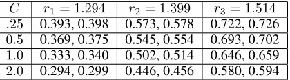
C r1= 1.294 r2= 1.399 r3= 1.514 .25 0.393, 0.398 0.573, 0.578 0.722, 0.726 0.5 0.369, 0.375 0.545, 0.554 0.693, 0.702 1.0 0.333, 0.340 0.502, 0.514 0.646, 0.659 2.0 0.294, 0.299 0.446, 0.456 0.580, 0.594 Table 1: (Mean, Median) loss for attackers with constraints

kδδδk ≤C1, C2, C3, C4andkθθθˆ−θθθtargetk2=r1, r2, r3.

models (50 in each shell). Note that it is unclear a priori what values are appropriate for radii. As such, we considered the (`2) distances between the 100θˆθθ’s and selectedr1as the

5-th percentile. That is, 5% of 5-the models are wi5-thinr1of any

particular model on average. We selectedr2andr3in a

simi-lar fashion using the25-th and50-th percentiles respectively. This yieldedr1= 1.294, r2= 1.399, r3= 1.514.

For eachvvv(i) _{and its associated time series and target}

models, we consider four attackers. Each is bound by ann -ball with radiusC1= 0.25, C2,0.5, C3= 1.0, C4= 2.0

re-spectively. That isC(i)_{={δδδ : kδδδk ≤C}

j}. For each of the

three attackers, we computed attacks against each of the 150 targets for each of the 100 series, yielding a total of 45,000 attacks. Each attacker ran projected gradient descent with step sizeη =.1and terminated when the greatest (absolute) difference between Alice’s loss on the current iteration and any of the past 10 iterations was less than 1/1000. Experi-ments were coded using NumPy (Oliphant 2006) and run on the Google Compute Engine platform. Results are shown in Table 1.

We note several observations, the first of which is the rel-ative scale of ther’s andC’s. Surprisingly, even with a rela-tively small change tokvvvkof up toC1 =.25, Alice is able

to shift Bob’s learned model byr1−.393 =.911on average

whenkθθˆθ−θθθtarget_{k = r}

1. Values for the other attackers are

of similar scale. What is perhaps most surprising, though, is the following observation seen in each of the four attack-ers: As the distance from Bob’s original model to Alice’s target increases fromr1tor2tor3, Alice’s loss increases at

a much faster rate. We posit that this could be explained by either Alice finding local minima in her search process or by a more intrinsic property of her loss as a function ofδδδ. We conjecture that if local minima were indeed the explanation then we would see a point where increasingC would stop yielding improved results. We note thatC1is substantially

smaller thanr1whileC4is larger thanr4, and yet we do not

see such a tapering-off in Alice’s loss. We therefore believe that local minima are not to blame and instead there is an-other, unknown, underlying phenomena at play. We intend to investigate this further in future work.

Related Work

Adversarial learning (Dalvi et al. 2004; Lowd and Meek 2005) studies the use of machine learning in the presence of intelligent adversaries. This includes data manipulation at-tacks at training time (as we study in this work) as well as de-ployment time attacks, defense strategies, and the construc-tion of learning algorithms robust to attacks. We direct the

reader to the recent surveys by Biggio and Roli (2018), and by Vorobeychik and Kantarcioglu (2018) for an overview of the field.

Most closely related to the work presented herein is the work of Mei and Zhu (2015) and Jagielski et al. (2018). Mei and Zhu also use a gradient-descent algorithm to attack lin-ear regression, and use the same KKT trick (also used by Biggio, Nelson, and Laskov, 2012 for training time attacks against Support Vector Machines and by Cauwenberghs and Poggio, 2001 in a non-adversarial context) to convert Al-ice’s bi-level optimization to a single-level program. In at-tacking linear regression at training time, however, Mei and Zhu restrict their attention to an attacker which can only af-fect target values, simplifying the gradient computation. In addition, their learner is not transforming the data prior to learning. Jagielski et al. attack linear regression in a setting where all target values are bounded between 0 and 1. They consider an attacker which adds arbitrary points (adhering to the bound on target values), which they capture by using the attacker adding initial points and the moving them based on the gradient of the loss.5_{Their attacker is unbounded in the} sense that it may add any point (but bounded in the number of points it can add) and as such, they have no need for the projection step of our attacker’s algorithm. To compute the attack, they compute the derivative of the attacker loss with respect to a single point’s features (but not its target value, which their attacker leaves constant) and use a coordinate-wise gradient descent algorithm. Our work unifies and gen-eralizes these two settings by computing the derivative of the attacker loss with respect to arbitrary additive perturbations to both features and target values. In addition, we require no bounds on the target values and can handle Bob performing a series of transformations prior to learning and after Alice’s attack. This generality is required in attacking autoregressive learners, and stems from our use of MDC.

Prior work has examined attacking (and defending) au-toregressive forecasters after learning has concluded at deployment time, whereas we focus on training-time at-tacks. Alfeld, Zhu, and Barford (2016) perform optimal deployment-time attacks against linear autoregressive mod-els where an attacker aims to draw the defender’s forecast to some target. In later work (Alfeld, Zhu, and Barford 2017), the authors defend linear models (including autoregressive forecasters) against such attackers with unknown targets by taking explicit defense actions. Separate from autoregres-sive models, others have investigated attacks on regression models at test time. Großhans et al. (2013) positions the in-terplay between attacker and defender as a Bayesian game while Tong et al. (2018) consider the setting with a single attacker and multiple learners. Our work complements prior work in that we examine attackers which perturb data during the learning phase, prior to when a model has been learned.

Related in spirit to ours is past work (Rubinstein et al. 2009; Xiao et al. 2015) which computes attacks against various forms of feature selection, and investigations of (possibly randomized) feature selection as a defense

strat-5

egy (Zhang et al. 2016; Alpcan, Rubinstein, and Leckie 2016). By contrast, ours is the first systematic approach to optimal best-response attacks to compositions of both pre-processing and learning. Pre-learning transformation has been highlighted in the literature as a potential challenge for attackers (Huang et al. 2011).

Conclusion

This paper contributes a framework based on matrix differ-ential calculus for attacking compositions of pre-processing transformations and learning. We consider the natural threat model wherein the attacker Alice perturbs original data (prior to the defender Bob transforming it) and then Bob learns on that data.

Our use of MDC delivers two key advantages. First, the resulting plug-and-play framework permits arbitrary com-position of differentiable learner and transform mappings. One can compute (matrix) derivatives of learner and trans-formindependently, and then multiply the results in order to compute the derivative of the composition. As such, our framework improves the applicability of known gradient-based attacks on learners — by phrasing the known deriva-tives in the MDC context, attacks can be extended to affect learners which first transform the data. Second, through al-gebraic manipulations of a matrix differential, we computed the derivative of OLS linear regression with respect to addi-tive changesin both features and target values. This extends the current state-of-the-art in training-time attacks against linear regression, which considers attackers perturbing ei-ther exclusively features or exclusively target values.

While attackers perturbing both features and target values are of independent interest of autoregressive forecasting, the Hankel transformation necessitates such an attacker model. We derive the (matrix) derivative of the Hankel transforma-tion, as well as the transform where a learner prepends a col-umn of1’s to account for a bias term. These, combined with the previously discussed plug-and-play nature of our frame-work, yield attacks against (in)homogeneous linear autore-gressive learners. Similarly, we derive the (matrix) derivative of the Vandermonde transform, extending the applicability of attacks against linear regression to polynomial regression. This work was supported by The Gregory S. Call Un-dergraduate Research Program at Amherst College and the Australian Research Council (DE160100584).

References

Alfeld, S.; Zhu, X.; and Barford, P. 2016. Data Poisoning Attacks against Autoregressive Models. InProceedings of the 30th Conference on Artificial Intelligence (AAAI 2016). Alfeld, S.; Zhu, X.; and Barford, P. 2017. Explicit De-fense Actions Against Test-Set Attacks. InProceedings of the 31th Conference on Artificial Intelligence (AAAI 2017), 1274–1280.

Alpcan, T.; Rubinstein, B. I. P.; and Leckie, C. 2016. Large-scale strategic games and adversarial machine learning. In

2016 IEEE 55th Conference on Decision and Control, CDC, 4420–4426. IEEE.

Barreno, M.; Nelson, B.; Sears, R.; Joseph, A. D.; and Tygar, J. D. 2006. Can machine learning be secure? InProceedings of the 2006 ACM Symposium on Information, Computer and

Communications Security, 16–25. ACM.

Biggio, B., and Roli, F. 2018. Wild patterns: Ten years after the rise of adversarial machine learning.Pattern Recognition

84:317–331.

Biggio, B.; Corona, I.; Maiorca, D.; Nelson, B.; ˇSrndi´c, N.; Laskov, P.; Giacinto, G.; and Roli, F. 2013. Evasion attacks against machine learning at test time. In Joint European Conference on Machine Learning and Knowledge Discovery in Databases, 387–402. Springer.

Biggio, B.; Nelson, B.; and Laskov, P. 2012. Poisoning attacks against support vector machines. In Langford, J., and Pineau, J., eds.,29th International Conference on Machine Learning (ICML), 1807–1814. Omnipress.

Bontempi, G.; Taieb, S. B.; and Le Borgne, Y.-A. 2012. Machine learning strategies for time series forecasting. In

European Business Intelligence Summer School, 62–77.

Springer.

Box, G. E.; Jenkins, G. M.; Reinsel, G. C.; and Ljung, G. M. 2015. Time series analysis: forecasting and control. John Wiley & Sons.

Cauwenberghs, G., and Poggio, T. 2001. Incremental and decremental support vector machine learning. InAdvances in Neural Information Processing Systems, 409–415. Dalvi, N.; Domingos, P.; Sanghai, S.; Verma, D.; et al. 2004. Adversarial classification. InProceedings of the Tenth ACM SIGKDD International Conference on Knowledge

Discov-ery and Data Mining, 99–108. ACM.

Großhans, M.; Sawade, C.; Br¨uckner, M.; and Scheffer, T. 2013. Bayesian Games for Adversarial Regression Prob-lems. Proceedings of the 30th International Conference on

Machine Learning28:55–63.

Huang, L.; Joseph, A. D.; Nelson, B.; Rubinstein, B. I. P.; and Tygar, J. D. 2011. Adversarial machine learning. In

Proceedings of the 4th ACM Workshop on Security and Ar-tificial Intelligence, 43–58. ACM.

Jagielski, M.; Oprea, A.; Biggio, B.; Liu, C.; Nita-Rotaru, C.; and Li, B. 2018. Manipulating machine learning: Poi-soning attacks and countermeasures for regression learning. In2018 IEEE Symposium on Security and Privacy (SP), 19– 35.

Lowd, D., and Meek, C. 2005. Adversarial learning. In Pro-ceedings of the Eleventh ACM SIGKDD international Con-ference on Knowledge Discovery in Data Mining, 641–647. ACM.

Magnus, J. R., and Neudecker, H. 1988. Matrix differen-tial calculus with applications in statistics and econometrics.

Wiley Series in Probability and Mathematical Statistics. Mei, S., and Zhu, X. 2015. Using Machine Teaching to Identify Optimal Training-Set Attacks on Machine Learn-ers. Twenty-Ninth AAAI Conference on Artificial

Intelli-gence2871–2877.

Rubinstein, B. I. P.; Nelson, B.; Huang, L.; Joseph, A. D.; Lau, S.-h.; Rao, S.; Taft, N.; and Tygar, J. D. 2009. ANTI-DOTE: Understanding and defending against poisoning of anomaly detectors. In Proceedings of the 9th ACM

SIG-COMM Conference on Internet Measurement, 1–14. ACM.

Szegedy, C.; Zaremba, W.; Sutskever, I.; Bruna, J.; Erhan, D.; Goodfellow, I.; and Fergus, R. 2013. Intriguing proper-ties of neural networks. arXiv preprint arXiv:1312.6199. Tong, L.; Yu, S.; Alfeld, S.; and Vorobeychik, Y. 2018. Ad-versarial regression with multiple learners. Proceedings of the 35th International Conference on Machine Learning. Vorobeychik, Y., and Kantarcioglu, M. 2018. Adversarial machine learning. Synthesis Lectures on Artificial

Intelli-gence and Machine Learning#38.

Xiao, H.; Biggio, B.; Brown, G.; Fumera, G.; Eckert, C.; and Roli, F. 2015. Is feature selection secure against training data poisoning? InInternational Conference on Machine Learning, 1689–1698.