522
Copyright © 2011-15. Vandana Publications. All Rights Reserved.
Volume-5, Issue-2, April-2015
International Journal of Engineering and Management Research
Page Number: 522-527
Control Strategy for Processes with Complex Dynamics
Sandeep Kumar Sunori1, Govind Singh Jethi2, Pradeep Kumar Juneja3
1,2
Department of ECE, Graphic Era Hill University, Bhimtal Campus, INDIA
3
School of Electronics,Graphic Era University,Dehradun,India
ABSTRACT
The processes which are found in various chemical industries have a complex dynamics in the sense that they are generally non linear, having dead time, inverse response and a severe multivariable interaction which makes the controlling of such processes difficult. In the present work an industrial process of first order with dead time is taken up as a case study for which controllers are designed incorporating dead time compensation and inverse response compensation techniques. The control performances of uncompensated and the compensated controllers are also compared.
Keywords— Inverse response, Smith predictor, Padé approximation, dead time.
I.
I
NTRODUCTIONThe general form of first order plus dead time (FODT)[6] system is,
.
Where K, α and τare process gain, time delay
and time constant respectively. In such process the effect of control action is reflected in the output after the time delay .Besides this, time delay incorporates a destabilizing effect also in the control system for such processes.
In the Bode diagram of a normal first order system without time delay, the phase angle asymptotically approaches a limiting value of -90 degrees thus never reaches the critical value of -180 degrees hence this system is always stable.
In contrast, in Bode diagram of FODT system, the phase angle decrease monotonically with frequency with no limits. There is now a limiting value of proportional controller gain at which the phase angle crosses -180 degrees and the system becomes unstable.
The higher the value of time delay, the smaller is this limiting value of controller gain.
The further analysis will be focused on a particular FODT process represented by relation (2) with the open loop step response shown in Fig.1. which clearly shows a time delay of 10 seconds in the response.
Fig.1.Open loop step response of FODT process
II.
PADÉ
APPROXIMATION
523
Copyright © 2011-15. Vandana Publications. All Rights Reserved.
Now the first, second and third orderPadé approximation of the considered process given by relation (2) using relations (3), (4) and (5) are specified in relations (6), (7) and (8) respectively.
The open loop step response of first order approximation of Gp
Fig 2.Open loop step response with first order Padéapproximation (green curve)
(s) is shown in Fig.2.
Higher is the order of approximation, closer will be that approximation to the actual transfer function. This can be easily verified from Fig.3 which clearly shows that the third order approximation best matches with the FODT process.
Fig 3.Comparision of Padé approximations (darkblue-FODT,green-approx.1,red-approx.2,lightblue-approx.3)
Now, we will design a PID controller for the FODT process with first order Padé approximation which is an inverse response system. This system is shown in Fig.4 with tuned values:
Kp=0.2083
Ki=0.0095
Kd
Fig 4. PID controller for Padé first order approximation
Here the plant is an inverse response system[2][3] of the form,
=-0.9563
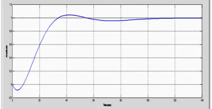
In case of such systems the controller first takes the wrong decision and the output moves in wrong direction as shown in Fig.5
524
Copyright © 2011-15. Vandana Publications. All Rights Reserved.
The characteristic parameters of this response are shown in Table 1.
Parameter Value
Rise time (sec) 18.2
Settling time (sec) 96.2
Overshoot (%) 4.23
Peak amplitude 1.04
Table 1. Characteristics of closed loop step response of PID controller for Padé first order approximation
III.
INVERSE
RESPONSE
COMPENSATION
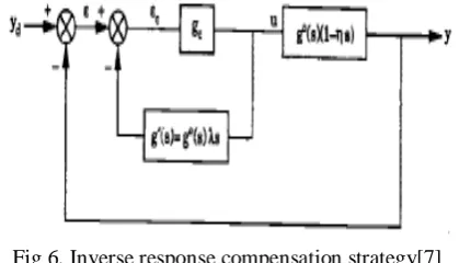
The block diagram of a controller with inverse response compensation is shown in Fig.6
Fig 6. Inverse response compensation strategy[7]
Here the plant is of the form given by relation (9) and the inner feedback path has the gain,
Where the parameter 𝜆𝜆>𝜂𝜂..
The choice 𝜆𝜆= 2𝜂𝜂 gives the optimum performance. The simulink model of the control system of Fig.4 incorporating inverse response compensation is shown in Fig.7 with tuned values,
Kp=0.31039
Ki=0.033127
Kd
Fig.7 PID controller incorporating inverse response compensation
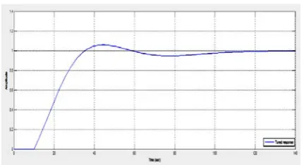
The closed loop step response of the modified PID controller of Fig.7 is shown in Fig.8 which clearly contains no inverse response.
=-1.0965
Fig 8. Closed loop step response of PID controller with inverse response compensation
The characterstic parameters of this response are specified in Table 2.
Parameter Value
Rise time (sec) 9.94
Settling time (sec) 34.2
Overshoot (%) 8.52
Peak amplitude 1.09
Table 2. Characteristics of closed loop step response of PID controller with inverse response compensation
525
Copyright © 2011-15. Vandana Publications. All Rights Reserved.
IV.
TIME DELAY COMPENSATION:
THE SMITH PREDICTOR
The undesired effects of the time delay can be nullified by incorporating smith predictor in the conventional control system. The block diagram of a controller incorporating smith predictor is shown in Fig. 9.The minor loop of Fig.9 is known as Smith predictor[4][5]. This scheme is designed for constant time delays and may therefore not perform as well for systems with time delays which vary significantly over time.
Fig 9. Control system with Smith predictor[7]
Here the plant has the form,
and the inner feedback path has the gain of the form,
Under no model errors,
The introduction of the minor loop eliminates the time delay factor from the feedback loop where it causes stability problems and move it outside of the loop where it has no effect on closed loop system stability.
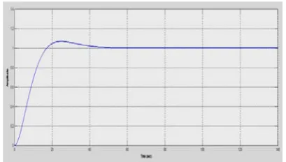
For the considered FODT process Gp(s), the
closed loop step response of the PID controller without time delay compensation with tuned values:
Kp=0.19664,
Ki=0.00893,
Kd
Fig 10. Closed loop step response of PID controller for FODT system
The characteristic parameters of this response are specified in Table 3.
=-1.18053
is shown in Fig.10.
Parameter Value
Rise time (sec) 18.4
Settling time (sec) 104
Overshoot (%) 5.92
Peak amplitude 1.06
Table 3. Characteristics of closed loop step response of PID controller for FODT system
Now the modified PID controller incorporating smith predictor with tuned values:
Kp=0.2637
Ki=0.0297
Kd
Fig.11 PID controller incorporating Smith predictor =-0.8206
is shown in Fig.11.
526
Copyright © 2011-15. Vandana Publications. All Rights Reserved.
Table 4 showing that there is a dramatic improvement in the performance after dead time compensation.
Fig 12. Closed loop step response of PID controller with Smith predictor
Parameter Value
Rise time (sec) 11.4
Settling time (sec) 40.1
Overshoot (%) 6.78
Peak amplitude 1.07
Table 4. Characteristics of closed loop step response of PID controller with Smith predictor
V.
EFFECTS OF MODEL
MISMATCH
The Smith predictor scheme will work perfectly as long as the process model is perfectly known. Modeling errors will definitely affect its performance. Thus this technique is very sensitive to modeling errors. Now we will investigate the effect of process gain errors, time delay errors and time constant errors separately on the Smith predictor performance retaining the same PI controller and Smith predictor[7]. The true process models taken up to expose the undesired effects of process gain perturbation, time delay perturbation and time constant perturbation are specified as a transfer function in relations (13),(14)and (15) respectively.
Now the closed loop step responses of same PID controller with same minor loop used in Fig.11 for these true models are presented in Fig.13 and the corresponding parameters are specified in Table 5, 6 and 7 respectively.
Fig 13. Smith predictor responses with model errors (red-gain error,blue-time delay error,pink-time constant
error)
Parameter Value
Rise time (sec) 11
Settling time (sec) 38.5
Overshoot (%) 11.8
Peak amplitude 1.12
Table 5. Smith predictor performance with process gain error
Parameter Value
Rise time (sec) 11.4
Settling time (sec) 40.1
Overshoot (%) 6.78
Peak amplitude 1.07
527
Copyright © 2011-15. Vandana Publications. All Rights Reserved.
Parameter ValueRise time (sec) 11.8
Settling time (sec) 49.5
Overshoot (%) 5.31
Peak amplitude 1.05
Table 7. Smith predictor performance with time constant error
The comparison of Table 4, 5, 6 and 7 indicates that there is no effect of the considered time delay perturbation in the response whereas the model errors caused by gain and time constant errors introduce significant degradation in the response.
VI.
CONCLUSION
The analysis done in the present work reveals that the higher is the value of order of Padé approximation, better will be the approximation of first order with dead time system function. The performance of the controllers for inverse response systems has been significantly improved using inverse response compensation technique. A significant cancellation of the degradation caused by the presence of time delay has been done incorporating Smith predictor in the control
system. It has also been observed that model errors have a significant undesirable effect in the performance of Smith predictor based control system.
REFERENCES
[1]Brezenski,C.,”Extrapolation algorithms and Padé approximations”,Applied Numerical Mathematics 20(3),299-318,1996.
[2]Waller,K.and C.Nygardas,”On Inverse Response in Process Control”,I&EC Fund.,14,221,1975.
[3]Iinoya,K.and R.J.Altpeter,”Inverse Response in Process Control,”I&EC,54,(7),39,1962.
[4]Smith,O.J.M.,”Close Control of Loops with Dead Time”,Chem.Eng.Prog.,53,(5),217,1957.
[5]Smith,O.J.M.,”A Controller to Overcome Dead Time”,ISA Journal,6,(2),28,1959.
[6]Paraskevopoulos,P.N;Pasgianos,G.D.and
Arvanitis,K.G.,”PID-Type Controller Tuning for Unstable First Order Plus DeadTime Processes Based on Gain and Phase Margin Specifications”,Control Systems Tecnology,IEEE Transactions,Vol.1,Issue 5,926-936,2006