The Thirty-Third AAAI Conference on Artificial Intelligence (AAAI-19)
Path-Specific Counterfactual Fairness
Silvia Chiappa
[email protected]DeepMind London
Abstract
We consider the problem of learning fair decision systems from data in which a sensitive attribute might affect the de-cision along both fair and unfair pathways. We introduce a counterfactual approach to disregard effects along unfair path-ways that does not incur in the same loss of individual-specific information as previous approaches. Our method corrects ob-servations adversely affected by the sensitive attribute, and uses these to form a decision. We leverage recent develop-ments in deep learning and approximate inference to develop a VAE-type method that is widely applicable to complex non-linear models.
Introduction
Machine learning is increasingly being used to take decisions that can severely affect people’s lives,e.g.in policing, educa-tion, hiring, lending, and criminal risk assessment (Hoffman, Kahn, and Li 2015; Dieterich, Mendoza, and Brennan 2016). This phenomenon has been accompanied by an increase in concern about disparate treatment caused by model errors and bias in the data.
In response to calls from governments and institutions, researchers have started to study how to ensure that learned models do no take decisions that areunfairwith respect to sensitive attributes(e.g.race and gender) using different ap-proaches. Among them, the causal framework (Pearl 2000; Dawid 2007; Pearl, Glymour, and Jewell 2016; Peters, Janz-ing, and Sch¨olkopf 2017) offers an intuitive and powerful way of reasoning about fairness, by viewing unfairness as the presence of an unfaircausal effectof the sensitive attribute on the decision (Qureshi et al. 2016; Bonchi et al. 2017; Kilbertus et al. 2017; Kusner et al. 2017; Russell et al. 2017; Zhang and Wu 2017; Zhang, Wu, and Wu 2017; Nabi and Shpitser 2018; Zhang and Bareinboim 2018).
Kusner et al. recently introduced a causal, individual-level, definition of fairness, calledcounterfactual fairness, which states that a decision is fair toward an individual if it coincides with the one that would have been taken in a counterfactual world in which the sensitive attribute were different. Counter-factual fairness assumes that the entire effect of the sensitive attribute on the decision is problematic. This is restrictive
Copyright c2019, Association for the Advancement of Artificial Intelligence (www.aaai.org). All rights reserved.
for scenarios in which the sensitive attribute might affect the decision along both fair and unfair pathways.
For example, in the case of Berkeley’s alleged sex bias in graduate admission (Pearl 2000), female applicants were rejected more often than male applicants as they were more often applying to departments with lower admission rates. Such an effect of gender through department choice is not
A Q
D Y
fair unfair
unfair as far as the college is concerned. What would be inad-missible is if the college treated male and female applicants with the same qualifications and applying to the same depart-ments differently because of gender. This complex scenario can be represented by the graphical causal model depicted above. In this model,A,Q,D, andY are random variables representing respectively gender, qualification, department choice, and admission decision,A→ D →Y is a causal path representing the influence of genderAon admission decisionY through department choiceD, andA→Y is a causal path representing the direct influence ofAonY.
To deal with such scenarios, we propose a novel defini-tion of fairness calledpath-specific counterfactual fairness, which states that a decision is fair toward an individual if it coincides with the one that would have been taken in a counterfactual world in which the sensitive attributealong the unfair pathwayswere different. In the Berkeley example, this would mean that an admission decision would be fair toward a female candidate if it would remain the same when pretending that the candidate were male alongA→Y.
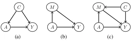
C
A Y
(a)
M
A Y
(b)
C M
A Y
(c)
Figure 1: (a): GCM with a confounderCfor the causal effect ofAonY. (b): GCM with one direct path and one indirect causal path fromAtoY. (c): GCM with a confounderCfor the causal effect ofMonY.
than previous approaches to path-specific fairness based on constraining the learning of the model parameters to eliminate or reduce unfair effects (Kilbertus et al. 2017; Nabi and Shpitser 2018).
Background on Causality
Causal relationships among random variables can visually be expressed usinggraphical causal models(GCMs). A GCM is a special case of a graphical model (see Chiappa for a quick introduction) that captures both independence and causal re-lations. In this work, we restrict ourselves todirected acyclic graphs,i.e.graphs in which a node cannot be anancestor of itself. In a directed acyclic graph, the joint distribution over all nodesp(X1, . . . , XI)is given by the product of the
conditional distributions of each nodeXigiven itsparents
pa(Xi),i.e.p(X1, . . . , XI) =Q I
i=1p(Xi|pa(Xi)).
GCMs enable us to give a graphical definition of causes and causal effects: if there exists adirected pathfromAto
Y, thenAis apotential causeofY. Directed paths are also calledcausal paths. The causal effect ofAonY can be seen as the information thatAsends toY through causal paths, or as the conditional distribution ofY givenArestricted to causal paths.
This implies that if there exist at least oneopennon-causal path betweenAandY then the causal effect ofAonY differs fromp(Y|A). An example of such a path isA ←C →Y
in the GCMG of Fig. 1(a): the variableC is said to be a confounderfor the effect ofAonY. In this case, the causal effect ofA = aonY can be seen as the conditional dis-tributionp→A=a(Y|A=a)on the modified GCMG→A=a,
resulting frominterveningonAby replacingp(A|C)with a delta distributionδA=a (thereby removing the link from
CtoA) and leaving the remaining conditional distributions
p(Y|A, C)andp(C)unaltered.
The rules of do-calculus (Pearl 2000; Pearl, Glymour, and Jewell 2016) indicate if and how the conditional distribu-tion in the intervened graph can be estimated using obser-vations fromG: if C is observed p→A=a(Y|A = a) = P
Cp(Y|A = a, C)p(C), whilst ifC is unobserved
esti-mating the conditional distribution using only observations fromGis not possible – in this case the effect is said to be non-identifiable.
We defineYA=ato be the random variable with distribution
p(YA=a) = p→A=a(Y|A = a). YA=a is called potential
outcomevariable and we will refer to it with the shorthand
Ya.
By performing different interventions onAalong different causal paths, it is possible to isolate the contribution of the causal effect ofAonY along a group of paths.
Direct and Indirect Effect. The simplest cases are the iso-lation of the contributions along the direct pathA→Y ( di-rect effect) and along the indirect causal pathsA→. . .→Y
(indirect effect).
Suppose that the GCM contains only one indirect causal path through a variableM, as in Fig. 1(b). We defineYa(Ma0)
to be the random variable that results from the interventions
A=aalongA→Y andA=a0alongA→M →Y. Theaverage direct effect(ADE) and theaverage indirect effect(AIE) ofA=awith respect toA=a0are given by1
ADE =hYa(Ma0)i − hYa0i, AIE =hYa0(Ma)i − hYa0i,
where,e.g.,hYai= R
YaYap(Ya).
More generally, the ADE ofA=awith respect toA=a0
can be estimated by computing the difference between 1) the average effect ofA=aalong the direct pathA →Y and
A=a0along the indirect causal pathsA→. . .→Y and 2) the average effect ofA=a0along all causal paths.
Similarly, the AIE ofA=awith respect toA=a0 can be estimated by computing the difference between 1) the average effect ofA=a0 along the direct pathA→Y and
A=aalong the indirect causal pathsA→. . .→Y and 2) the average effect ofA=a0along all causal paths.
Under the independence assumptionYa,m⊥⊥Ma0(
sequen-tial ignorability),p(Ya(Ma0))can be estimated as
p(Ya(Ma0)) = Z
m
p(Ya(Ma0)|Ma0 =m)p(Ma0 =m)
=
Z
m
p(Ya,m|Ma0 =m)p(Ma0 =m)
=
Z
m
p(Ya,m)p(Ma0 =m), (1)
where to obtain the second line we have used the consis-tencyproperty (Pearl, Glymour, and Jewell 2016). As there are no confounders, intervening coincides with condition-ing,i.e. p(Ya,m) = p(Y|A = a, M = m)andp(Ma0) =
p(M|A=a0).
If the GCM contains a confounder for the effect of eitherA
orMonY, such asCin Fig. 1(c), thenp(Ya,m)6=p(Y|A=
a, M =m). In this case, by following similar arguments as the ones used in Eq. (1) but conditioning onC(and therefore assumingYa,m⊥⊥Ma0|C), we obtain2
p(Ya(Ma0)) = Z
m,c
p(Y|a, m, c)p(m|a0, c)p(c).
IfCis unobserved, the effect is non-identifiable.
1
In this paper, we consider thenaturaleffect, which generally differs from thecontrolledeffect; the latter corresponds to interven-ing onM.
2
Path-Specific Effect. In the more complex case in which, rather than computing the direct and indirect effects, we want to isolate the contribution of the effect along a specific group of paths, we can generalize the formulas for the ADE and AIE by using in the first term the variable resulting from performing the interventionA=aalong the group of interest andA=a0along the remaining causal paths.
For example, consider the GCM of Fig. 2 and assume that we are interested in isolating the effect of A onY along the direct pathA → Y and the paths passing throughM,
A→M →, . . . ,→Y, namely along the green and dashed green-black links. Thepath-specific effect(PSE) ofA=a
with respect toA=a0for this group of paths is given by
PSE =hYa(Ma, La0(Ma))i − hYa0i,
wherep(Ya(Ma, La0(Ma)))can be computed as
Z
c,m,l
p(Y|a, c, m, l)p(l|a0, c, m)p(m|a, c)p(c).
In the simple case in which the GCM corresponds to a linear model,e.g.
A∼Bernoulli(π), C=c,
M =θm+θamA+θmc C+m,
L=θl+θlaA+θclC+θml M+l,
Y =θy+θyaA+θcyC+θymM +θylL+y, (2)
where c,m,l andy are unobserved independent
zero-mean Gaussian terms, we have
hYa(Ma, La0(Ma))i=θy+θymθm+θy l(θ
l+θl mθ
m)
+θaya+θmyθmaa+θly(θlaa0+θml θma a).
The PSE is therefore given by
θya(a−a0) +θ y mθ
m
a (a−a0) +θ y lθ
l mθ
m
a (a−a0). (3)
Shpitser gives a recursive rule for obtaining the variable of interest for computing the PSE, and a graphical method for understanding whether the PSE is identifiable in the presence of unobserved confounders.
Path-Specific Counterfactual Fairness
We are interested in complex scenarios in which the sensitive attributeAmight affect the decision variableY along both fair and unfair causal pathways. We assume thatAcan only take two valuesaanda0, and thata0is a baseline value.Kilbertus et al. and Nabi and Shpitser propose to deal with such scenarios by constraining the learning of the model parameters such that the average of the unfair effect is elimi-nated or reduced. More specifically, Nabi and Shpitser sug-gest to perform model training by constraining the unfair PSE ofAonY to lie in a small range. The main limitation of this approach is that, at test time, it requires averaging over all variables that are descendants of the sensitive attribute through the unfair causal pathways. This can negatively im-pact the system’s predictive accuracy, as individual-specific information about those descendants is disregarded. Kilbertus et al. propose to directly identify a set of constraints on the
C
A M L Y
Figure 2: GCM corresponding to Eq. (2).
conditional distribution of the decision variable that eliminate the unfair effect. This can easily be done in linear models, but it is unclear how to identify the constraints in more complex non-linear scenarios. Furthermore, this approach also unnec-essarily removes information from problematic descendants. In contrast, we propose to simplycorrectat test time the decisions of individuals for whichA = aby making sure that they coincide with the one that would have been taken in a counterfactual world in which the sensitive attribute along the unfair pathways were set to the baseline. This re-quires correcting the observations corresponding to variables that are descendants of the sensitive attribute through unfair pathways, by removing the unfair information induced by the sensitive attribute while retaining the remaining fair in-formation. We achieve this through a generalization of the abduction-action-prediction method for counterfactual rea-soning (Pearl 2000). We generally refer to our approach as path-specific counterfactual fairness(PSCF). For the Berke-ley alleged sex bias case for example, PSCF would ensure that the admission decision of a female applicant coincides with the one that would have been taken in a counterfactual world in which her genderawere malea0along the direct pathA→Y, by taking a decision based on the intervention
A=a0alongA→Y.
To highlight its relation with the approaches of Kilbertus et al. and of Nabi and Shpitser, we first explain PSCF for the case in which the data-generation mechanism is given by the linear model of Eq. (2) (Fig. 2). Assume that the direct effect ofAonY and the effect throughM are con-sidered unfair. PSCF corrects the decision of an individual for whichA = aby performing the interventionA = a0
along the direct pathA→Y and the paths passing through
M, A → M →, . . . ,→ Y, namely along the green and dashed green-black links of Fig. 2. (Notice that the dashed green-black links differ fundamentally from the green links; they contain unfairness only as a consequence ofA→M, corresponding to the parameterθm
a , being unfair.) More
pre-cisely, assuming that a0 = 0 is the baseline value of A, given an instance{an =a = 1, cn, mn, ln}, the PSCF
ap-proach computes a fair predictionyn
PSCF ofy
nas the mean
ofp(Ya0(Ma0, La(Ma0))|a, cn, mn, ln). This is achieved by
first computingn
mandnl froma
n, cn, mn, lnand the model
equations (abduction),i.e.
nm=mn−θm−θma −θmc cn,
nl =θl−θla−θlccn−θlmmn.
Then fair transformations ofmnandln,mn
PSCFandl
n
PSCF, and
the fair predictionynPSCFare obtained by substitutingnmand
n
l into the model equations with the problematic termsθ m a
along the direct pathA→Y and the paths passing through
M,A→M →, . . . ,→Y),i.e.
mnPSCF=θm+ θ
m a +θ
m c c
n+n m,
lnPSCF=θl+θal +θlccn+θlmmnPSCF+nl ,
ynPSCF=θy+θya+θyccn+θmymnPSCF+θyllnPSCF. (4)
This approach can be seen as performing a correction on the decision through a correction on all the variables that are descendants of the sensitive attribute along unfair pathways (UP), namelyM andLin this case.
To understand the relation with thefair inference on out-comes(FIO) method suggested by Nabi and Shpitser, the PSE for this model (Eq. (3)) witha= 1anda0= 0takes the form
PSE=θya+θma (θmy +θylθlm).
FIO consists in performing a constrained learning of the model parameters θ such that the PSE lies in a small range. After training, a predictionyn
FIOofynfor an instance
{an, cn, mn, ln}can be obtained asyn
FIO = hYip(Y|an,cn),
wherep(Y|an, cn)is given by
Z
m,l
p(Y|an, cn, m, l)p(l|an, cn, m)p(m|an, cn),
i.e.as
mnFIO= ˆθm+ ˆθaman+ ˆθcmcn,
lnFIO= ˆθl+ ˆθlaan+ ˆθclcn+ ˆθml mnFIO,
ynFIO= ˆθy+ ˆθayan+ ˆθcycn+ ˆθymmnFIO+ ˆθyllnFIO,
whereθˆindicate the learned model parameters.
Assume that, at the end of training,θˆfor both PSCF and FIO coincide with the true underlying parametersθ, except for θˆma and θˆya in FIO which are assigned zero values to satisfy the constraint PSE = 0. Then, given an instance {an =a= 1, cn, mn, ln}, we can expressyPSCFn asynPSCF= hYip(Y|an,cn,mn,ln)−PSE, since
ynPSCF=θy+θyccn+θmymn+θylln−θma (θmy +θylθlm) ;
andynFIOasyFIOn =hYip(Y|an,cn)−PSE, since
yFIOn =θy+θyccn+θmym¯n+θly¯ln−θma (θmy +θlyθlm),
where m¯n = hMi
p(M|an,cn) = θm+θma +θmc cn. This
formulation highlights the disadvantage of FIO over PSCF in disregarding specific information about the individual,n
m
and n
l, through the use ofm¯
n and ¯ln. As the constraint
PSE= 0is not necessarily achieved by assigning zero values toθˆm
a andθˆay, this correspondence does not generally hold.
As the reason for averaging overM andL, Nabi and Sh-pitser indicate the need to account for the constraints that are potentially imposed onθˆm
a andθˆlm. If a constraint is imposed
on a parameter, then the corresponding variable needs indeed to be integrated out to ensure that such a constraint is taken into account in the prediction. For any model, the PSE would contain the parameters corresponding to the UP descendants
-10 -5 0 5 10
A=0 A=1
(a)
Hm C Hl
A M L Y
(b)
Figure 3: (a): Empirical distribution of the estimate ofn mfor
the case in whichmnis generated by Eq. (2) with an extra
non-linear termf(A, C)(continuous lines). Histograms of ˜
p(Hm|A)(crossed lines). (b): GCM with an explicit latent
variable for each UP descendant ofA.
ofA, which means that FIO would always require integrating out the UP descendants. However, even if we a priori identify a set of constraints that give PSE= 0, the UP descendants must be integrated out or corrected from unfairness even if no constraints are imposed on the corresponding parame-ters. Consider the case discussed above, where we achieve PSE= 0by settingθˆma andθˆyato zero values. This does not
constrainθˆl
m. However, to form a prediction ofyn, we would
still need to integrate overL, as the observationlncontains the problematic termθlyθl
mθam, corresponding to the unfair
part of the effect ofAonL.
In this simple case, we could avoid having to integrate overM andLby a priori imposing the constraintsθˆy
a = 0
andθˆy m=−θˆ
y lθˆ
l
m,i.e.by constraining the conditional
dis-tribution used to form a prediction ofyn,p(Y|A, C, M, L).
This coincides with the constraint proposed by Kilbertus et al. to avoid proxy discrimination. However, this approach achieves removal of the problematic unfairness inmnandln
by cancelling out the entiremnfrom the prediction. This is also suboptimal, as all information withinmnis disregarded.
Furthermore, it is not clear how to extend this approach to more complex scenarios.
In conclusion, the main advantage of our approach is that it allows to retain fair individual-specific information contained in the UP descendants. This is achieved by leaving unaltered the underlying data-generation mechanism during training.
Model-Observations Mismatch. Whilst offering several advantages over previous approaches to path-specific fairness, in the presence of a strong mismatch between the assumed and actual data-generation mechanisms, the PSCF approach described above would most likely not remove unfairness completely.
Indeed, in this case the estimates ofn
mandnl would not
be independent from the sensitive attributeA. Consider, for example, the case in which we assume the data-generation process of Eq. (2), but the observedmn,n= 1, . . . , N, are generated from a modified version of Eq. (2) containing an extra non-linear termf(A, C). The learned model parameters ˆ
it dependent onA, as shown in Fig. 3(a) (continuous lines). To solve this issue, we propose to decomposeminto two
components,i.e.m =Hm+ηm, and to adopt a training
procedure in whichp˜(Hm|A=a), defined as
˜
p(Hm|A=a) =
1
Na Na
X
n=1
p(Hm|an=a, cn, mn, ln) (5)
whereNa indicates the number of observations for which
an=a, is encouraged to have small dependence onA. We
can then use,e.g., the mean ofp(Hm|an, cn, mn, ln), rather
than the estimate ofn
m. In other words, we make sure that,
when estimating the latent randomness associated with an individual, we only pick up the part that does not depend on
A, and only use this part to perform the prediction.
Encouraging independence onAis necessary, as otherwise the estimatedp˜(Hn
m|A)would be close to the estimate of
n
m. This is shown by the histograms ofp˜(Hm|A)in Fig. 3(a)
(crossed lines), obtained by assuming a Gaussian distribution forp(Hm)and by learning the model parameters using an
expectation maximization approach.
To more generally ensure that the abduction procedure will not end up with estimates that depend on the sensitive variable, we need to encourage latent independence onAfor each descendant ofAthat needs to be corrected, namely for each UP descendant, and therefore introduce another latent variable forL,Hl(see Fig. 3(b)).
We propose a way to encourage independence onA to-gether with a method that generalizes the PSCF approach described above to complex non-linear models in the next section.
PSCF-VAE
Consider more general equations for the GCM of Fig. 3(b), given by
A∼Bernoulli(π), C∼pθ(C),
Hm∼pθ(Hm), M ∼pθ(M|A, C, Hm),
Hl∼pθ(Hl), L∼pθ(L|A, C, M, Hl),
Y ∼pθ(Y|A, C, M, L), (6)
where ifM is categorical we assumepθ(M|A, C, Hm) =
fθ(A, C, Hm), where fθ(A, C, Hm) can be any function
(e.g.a neural network); whilst ifM is continuous we assume thatpθ(M|A, C, Hm)is Gaussian with meanfθ(A, C, Hm).
The model likelihoodpθ(A, C, M, L, Y), and the posterior
distributions pθ(Hm|A, C, M, L) and pθ(Hl|A, C, M, L)
required to form fair predictions, are generally intractable. We address this issue with a variational approach that computes Gaussian approximations qφ(Hm|A, C, L, M)
and qφ(Hl|A, C, L, M) of pθ(Hm|A, C, M, L) and
pθ(Hl|A, C, M, L) respectively, parametrized by φ, as
discussed in detail below.
After learningθandφ, analogously to Eq. (4), we compute a fair predictionyn
PSCFfor an instance{an=a, cn, mn, ln}
ashYa0(Ma0, La(Ma0))ip(Y
a0(Ma0,La(Ma0))|a,cn,mn,ln),
esti-mated using a Monte-Carlo approach. Specifically, we first draw samples hn,im ∼ qφ(Hm|a, cn, mn, ln) and hn,il ∼
qφ(Hl|a, cn, mn, ln), fori= 1, . . . , I, and then form
mn,iPSCF∼pθ(M|a0, cn, hn,im),
ln,iPSCF∼pθ(L|a, cn, mn,iPSCF, h
n,i l ),
yPSCFn =1
I
I X
i=1 hYip
θ(Y|a0,cn,mn,iPSCF,l
n,i
PSCF)
. (7)
In the experiments, we usedI= 500.
If we group the observed and latent variables as V = {A, C, M, L, Y} and H = {Hm, Hl} respectively, the
variational approximationqφ(H|V)to the intractable
pos-terior pθ(H|V) is obtained by finding the variational
pa-rametersφthat minimize the Kullback-Leibler divergence KL(qφ(H|V)||pθ(H|V)). This is equivalent to maximizing
a lower boundFθ,φ on the log of the marginal likelihood
logpθ(V)≥ Fθ,φwith
Fθ,φ=−hlogqφ(H|V)iqφ(H|V)+hlogpθ(V, H)iqφ(H|V),
where,e.g.,
hlogqφ(H|V)iqφ(H|V)=
Z
H
qφ(H|V) logqφ(H|V).
In our case, rather thanqφ(H|V), we useqφ(H|V∗≡V\Y).
Our approach is therefore to learn simultaneously the latent embedding and predictive distributions in Eq. (7). This could be preferable to other causal latent variable approaches such as the FairLearning algorithm proposed by Kusner et al., which separately learns a predictor ofY using samples from the previously inferred latent variables and from the non-descendants ofA.
In order for Fθ,φto be tractable conjugacy is required,
which heavily restricts the family of models that can be used. This issue can be addressed with a Monte-Carlo approxi-mation known as variational auto-encoding (VAE) (Kingma and Welling 2014; Rezende, Mohamed, and Wierstra 2014). This approach representsHas a non-linear transformation
H =fφ(E)of a random variableEfrom a parameter free
dis-tributionq. As we chooseqto be Gaussian,H=µφ+σφE
withq=N(0,1)for the univariate case. This enables us to
rewrite the bound as
Fθ,φ=−hlogqφ(H=fφ(E)) + logpθ(V, H=fφ(E))iq.
The first part of the gradient of Fθ,φ with respect to φ, ∇φFθ,φ, can be computed analytically, whilst the second
part is approximated by
h∇φlogpθ(V, H=fφ(E))iq≈
1
I
I X
i=1
∇φlogpθ(V, hi=fφ(i)), i∼q.
In the experiments, we usedI= 1, as commonly done in the VAE literature. The variational parametersφare parametrized by a neural network taking as inputV∗.
Independence onA. In order to ensure thatq˜φ(H|A),
Hm C Hl Hr
A M L R Y
S A
C
R Hs
Y
Figure 4: (a): GCM for the UCI Adult dataset. (b): GCM for the UCI German Credit dataset.
2016) and with amaximum mean discrepancy(MMD) penal-ization approach (Gretton et al. 2012; Louizos et al. 2016), which gave similar but more stable results. The MMD ap-proach adds a penalty term to the boundFθ,φ,
−βLMMD(a, a0),
whereβis a weighting factor that determines the degree of independence, and therefore might correspond to different levels of fairness.LMMD(a, a0)is the sum of several terms,
one for each latent variable, wheree.g.the term forHmis
given by
Lm
MMD(a, a 0
) = 1 N2
a Na
X
i=1 Na
X
j=1
k(ha,im, h a,j m)
+ 1 N2
a0 Na0
X
i=1 Na0
X
j=1
k(ham0,i, h a0,j m )−
2 NaNa0
Na
X
i=1 Na0
X
j=1
k(ha,im, h a0,j m ),
wherekis a Gaussian kernel, andha,i
m is a sample from the
variational distribution for an individual for whichA=a.
Experiments
We evaluate the proposed PSCF-VAE method on the UCI Adult and German Credit datasets.
As prior distributionpθfor each latent variable (Eq. (6))
we used a ten-dimensional Gaussian with diagonal covari-ance matrix, whilst asfθwe used a neural network with one
linear layer of size 100 with tanh activation, followed by a linear layer (the outputs were Gaussian means for continuous variables and logits for categorical variables). As variational distributionqφwe used a ten-dimensional Gaussian with
di-agonal covariance, with means and log variances obtained as the outputs of a neural network with two linear layers of size 20 and tanh activation, followed by a linear layer. Train-ing was achieved with the Adam optimizer (KTrain-ingma and Ba 2015) with learning rate 0.01, mini-batch size 128, and de-fault valuesβ1 = 0.9,β2= 0.999, and= 1e-8. Training
was stopped after 20,000 steps.
The UCI Adult Dataset
The Adult dataset from the UCI repository (Lichman 2013) contains 14 attributes including age, working class, educa-tion level, marital status, occupaeduca-tion, relaeduca-tionship, race, gen-der, capital gain and loss, working hours, and nationality for 48,842 individuals; 32,561 and 16,281 for the training and test sets respectively. The goal is to predict whether the individual’s annual income is above or below $50,000. We assumed the GCM of Fig. 4(a) (following Nabi and Shpitser),
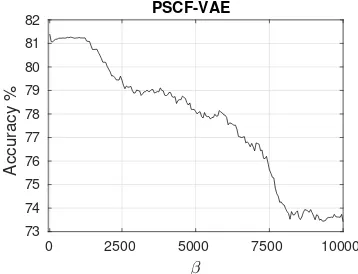
0 2500 5000 7500 10000
73 74 75 76 77 78 79 80 81 82
Accuracy %
PSCF-VAE
Figure 5: Test accuracy of PSCF-VAE on the UCI Adult dataset for increasing values ofβ.
whereAcorresponds to the protected attribute sex,Cto the duple age and nationality,M to marital status, Lto level of education,Rto the triple working class, occupation, and hours per week, andY to the income class3. Age, level of education and hours per week are continuous, whilst sex, nationality, marital status, working class, occupation, and income are categorical. Besides the direct effectA→Y, the effect ofAonY through marital status, namely along the pathsA→M →, . . . ,→Y, is considered unfair.
Nabi and Shpitser assume that all variables are contin-uous, exceptA andY, and linearly related, exceptY for whichp(Y = 1|pa(Y)) =π=σ(θy+P
Xi∈pa(Y)θ
y xiXi)
where σ(·) is the sigmoid function. With the encoding
A ∈ {0,1}, where 0 indicates the male baseline value, and under the approximation log(π/(1 − π)) ≈ logπ, we can write the PSE in the odds ratio scale as PSE ≈ exp(θy
a +θymθam+θ y lθ
l
mθma +θyr(θrmθam+θrlθ l
mθam)). An
instance from the test set {an, cn, mn, ln, rn} is classi-fied by using p(Y|an, cn) = R
m,l,rp(Y|a
n, cn, m, l, r)×
p(r|an, cn, m, l)p(l|an, cn, m)p(m|an, cn).
In Fig. 5, we show the accuracy obtained by PSCF-VAE on the test set for increasing values ofβ, ranging fromβ= 0(no MMD penalization) toβ= 10,000. As we can see, accuracy decreases from 81.2% to 73.4%. Notice that predictions were formed using samples of Hm, Hl andHr also for males,
even if not required. Also notice that forming predictions frompθ(Y|an, cn, mn, ln, rn)gives 82.7% accuracy.
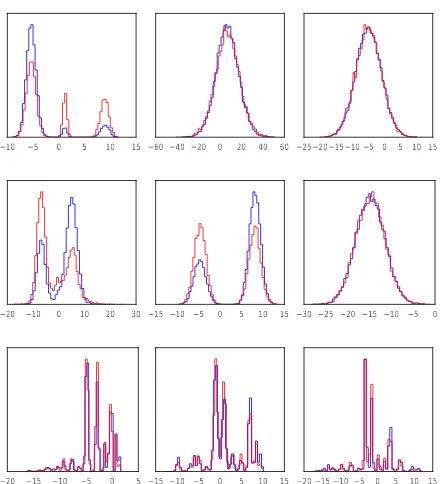
In Fig. 6, we show histograms of two dimensions of ˜
qφ(Hm|A) (first and second row) and one dimension of
˜
qφ(Hl|A)(third row) forβ= 0,β= 2,500, andβ= 5,000
(left to right) after 20,000 training steps for females (red) and males (blue) – these are the only variables that show differ-ences between male and females. As we can see, increasingβ
induces a reduction in the number of modes in the posterior, which corresponds to information loss. Forβ= 10,000all histograms are unimodal (not shown). Forβ = 5,000, for which accuracy is around 78%, the histograms for females
3
10 5 0 5 10 15 60 40 20 0 20 40 60 25 20 15 10 5 0 5 10 15
20 10 0 10 20 30 15 10 5 0 5 10 15 30 25 20 15 10 5 0
20 15 10 5 0 5 15 10 5 0 5 10 15 20 15 10 5 0 5 10 15
Figure 6: Histograms of two dimensions ofq˜φ(Hm|A)(first
and second row) and one dimension ofq˜φ(Hl|A)(third row)
forβ = 0,β = 2,500, andβ = 5,000(left to right) after 20,000 training steps for females (red) and males (blue).
and males are similar – this can therefore be considered a fair accuracy.
The unconstrained PSE on this dataset is 3.64. When con-straining the PSE to be smaller than 3.7 (thus essentially imposing no constraint), FIO gives 73.8% accuracy, due the information that is lost by integrating outM, LandR. Con-straining the PSE to be smaller than 3.6 also gives 73.8% accuracy. Constraining the PSE to be smaller than 1.05, as suggested by Nabi and Shpitser, gives 73.4% accuracy (Nabi and Shpitser report 72%). These results demonstrate that loss in accuracy in FIO is due to integrating out M, LandR, rather than to ensuring fairness.
The UCI German Credit Dataset
The German Credit dataset from the UCI repository contains 20 attributes of 1,000 individuals applying for loans. Each applicant is classified as a good or bad credit risk,i.e. as likely or not likely to repay the loan. We assume the GCM in Fig. 4(b), whereAcorresponds to the protected attribute sex,
Cto age,Sto the triple status of checking account, savings, and housing, andRthe duple credit amount and repayment duration. The attributes age, credit amount, and repayment duration are continuous, whilst checking account, savings, and housing are categorical. Besides the direct effectA→Y, we would like to remove the effect ofAonY throughS. We only need to introduce a hidden variableHsforS, asRdoes
not need to be corrected.
We divided the dataset into training and test sets of sizes 700 and 300 respectively. As for the Adult dataset, we varied
βfrom 0 to 10,000. The test accuracy remained 76.0% for
5 4 3 2 1 0 1 2 3 4 8 6 4 2 0 2 4 6 8
Figure 7: Histograms ofq˜φ(Hs|A)for one dimension of the
variable housing forβ = 0 andβ = 10,000after 20,000 training steps for females (red) and males (blue).
all values ofβ (predictions were formed using samples of
Hsalso for males). This is same accuracy obtained when
forming predictions frompθ(Y|an, cn, sn, rn).
In Fig. 7, we showq˜φ(Hs|A)for one dimension of the
variable housing, which shows the most significant difference between females and males, forβ= 0andβ = 10,000.
Conclusions
We have proposed a novel intuitive definition of fairness, path-specific counterfactual fairness, which states that a decision is fair toward an individual if it coincides with the one that would have been taken in a counterfactual world in which the sensitive attribute along the unfair pathways were different.
We have introduced a latent inference-projection method, PSCF-VAE, that achieves path-specific counterfactual fair-ness by correcting the variables that are descendants of the sensitive attribute along unfair pathways during testing, leav-ing unaltered the underlyleav-ing data-generation mechanism dur-ing traindur-ing. The proposed method is widely applicable to complex non-linear models.
PSCF-VAE requires providing the causal model underly-ing the data generation process. Future work will consider relaxing this requirement.
Acknowledgements
The author would like to thank Thomas P. S. Gillam for his contribution to this work.
References
Bonchi, F.; Hajian, S.; Mishra, B.; and Ramazzotti, D. 2017. Exposing the probabilistic causal structure of discrimination. International Journal of Data Science and Analytics3(1):1– 21.
Chiappa, S. 2014. Explicit-duration Markov switching mod-els. Foundations and Trends in Machine Learning7(6):803– 886.
Dawid, P. 2007. Fundamentals of statistical causality. Tech-nical report, University Colledge London.
Edwards, H., and Storkey, A. 2016. Censoring representa-tions with an adversary. In4th International Conference on Learning Representations.
Gretton, A.; Borgwardt, K.; Rasch, M.; Sch¨olkopf, B.; and Smola, A. 2012. A kernel two-sample test. Journal of Machine Learning Research13:723–773.
Hoffman, M.; Kahn, L.; and Li, D. 2015. Discretion in hiring.
Kilbertus, N.; Rojas-Carulla, M.; Parascandolo, G.; Hardt, M.; Janzing, D.; and Sch¨olkopf, B. 2017. Avoiding discrim-ination through causal reasoning. InAdvances in Neural Information Processing Systems 30, 656–666.
Kingma, D., and Ba, J. 2015. Adam: A method for stochastic optimization. In3rd International Conference on Learning Representations.
Kingma, D., and Welling, M. 2014. Auto-encoding varia-tional Bayes. In2nd International Conference on Learning Representations.
Kusner, M.; Loftus, J.; Russell, C.; and Silva, R. 2017. Coun-terfactual fairness. InAdvances in Neural Information Pro-cessing Systems 30, 4069–4079.
Lichman, M. 2013. UCI machine learning repository.
Louizos, C.; Swersky, K.; Li, Y.; Welling, M.; and Zemel, R. 2016. The variational fair autoencoder. In4th International Conference on Learning Representations.
Nabi, R., and Shpitser, I. 2018. Fair inference on outcomes. InThirty-Second AAAI Conference on Artificial Intelligence.
Pearl, J.; Glymour, M.; and Jewell, N. 2016.Causal Inference in Statistics: A Primer. Wiley.
Pearl, J. 2000. Causality: Models, Reasoning, and Inference. Cambridge University Press.
Peters, J.; Janzing, D.; and Sch¨olkopf, B. 2017. Elements of Causal Inference: Foundations and Learning Algorithms. MIT Press.
Qureshi, B.; Kamiran, F.; Karim, A.; and Ruggieri, S. 2016. Causal discrimination discovery through propensity score analysis.ArXiv e-prints.
Rezende, D.; Mohamed, S.; and Wierstra, D. 2014. Stochas-tic backpropagation and approximate inference in deep gen-erative models. In Proceedings of the 31st International Conference on Machine Learning, 1278–1286.
Russell, C.; Kusner, M.; Loftus, J.; and Silva, R. 2017. When worlds collide: Integrating different counterfactual assump-tions in fairness. InAdvances in Neural Information Process-ing Systems 30, 6417–6426.
Shpitser, I. 2013. Counterfactual graphical models for lon-gitudinal mediation analysis with unobserved confounding. Cognitive Science37(6):1011–1035.
Zhang, J., and Bareinboim, E. 2018. Fairness in decision-making – the causal explanation formula. InProceedings of the 32nd AAAI Conference on Artificial Intelligence.
Zhang, L., and Wu, X. 2017. Anti-discrimination learning: a causal modeling-based framework.International Journal of Data Science and Analytics1–16.