Boosted Kernel Ridge Regression: Optimal Learning Rates
and Early Stopping
Shao-Bo Lin [email protected]
Department of Mathematics Wenzhou University Wenzhou, China
Yunwen Lei [email protected]
Department of Computer Science and Engineering Southern University of Science and Technology Shenzhen, China
Ding-Xuan Zhou [email protected]
School of Data Science and Department of Mathematics City University of Hong Kong
Kowloon, Hong Kong, China
Editor:Arthur Gretton
Abstract
In this paper, we introduce a learning algorithm, boosted kernel ridge regression (BKRR), that combinesL2-Boosting with the kernel ridge regression (KRR). We analyze the learning
performance of this algorithm in the framework of learning theory. We show that BKRR provides a new bias-variance trade-off via tuning the number of boosting iterations, which is different from KRR via adjusting the regularization parameter. A (semi-)exponential bias-variance trade-off is derived for BKRR, exhibiting a stable relationship between the generalization error and the number of iterations. Furthermore, an adaptive stopping rule is proposed, with which BKRR achieves the optimal learning rate without saturation.
Keywords: learning theory, kernel ridge regression, boosting, integral operator
1. Introduction
Supervised learning aims at learning function relationships between input and output vari-ables, based on input-output pair samples. Kernel ridge regression (KRR) is a classical and standard approach for supervised learning due to its easy implementation and theoretical optimality (Evgeniou et al., 2000; Caponnetto and De Vito, 2007; Steinwart et al., 2009; Lin et al., 2017) and thus has triggered enormous research activities in the statistical and machine learning communities (Bauer et al., 2007; Caponnetto and De Vito, 2007; Cucker and Zhou, 2007; Smale and Zhou, 2007; Steinwart et al., 2009; Lin et al., 2017). However, KRR suffers from a so-called saturation phenomenon (Gerfo et al., 2008) meaning that its learning rate cannot be improved once the target (regression) function goes beyond a certain level of regularity. Furthermore, there lacks efficient parameter-selection strategies for KRR to realize its theoretically optimal learning performance. Many users’ spirit is dampened by these drawbacks and then turns to other learning algorithms such as the kernel-based
c
gradient descent (Yao et al., 2007), kernel-based conjugate gradient descent (Blanchard and Kr¨amer, 2016) and kernel-based partial least squares (Lin and Zhou, 2018b).
Boosting, originally proposed by Schapire (1990); Freund (1995), is devoted to producing a strong composite learner from a given class of weak learners. Some boosting algorithms can be interpreted from a viewpoint of statistical gradient descent to solve optimization problems with different loss functions (Friedman et al., 2000; Friedman, 2001). In this way, a special boosting algorithm, L2-Boosting, was interpreted as an iterative least squares fitting of residuals (Friedman, 2001; B¨uhlmann and Yu, 2003). L2-Boosting was utilized by Park et al. (2009) to improve the learning performance of Nadaya-Watson kernel estimators by overcoming saturation and was also proved in B¨uhlmann and Yu (2003) to be almost over-fitting resistant by exhibiting its exponential bias-variance trade-off for linear regression, reducing the difficulty of model selection.
The aim of this paper is to combine L2-Boosting with KRR to overcome the saturation and reduce the difficulty of model selection of KRR. Let (HK,k · kK) be the reproducing
kernel Hilbert space (RKHS) induced by a Mercer kernel K on a metric (input) space X
and D={(xi, yi)}Ni=1 ⊂ X × Y be a sample with Y ⊆Rthe output space. KRR is defined
by
fD,λ(1) := arg min
f∈HK
1
|D|
X
(x,y)∈D
(f(x)−y)2+λkfk2K
, (1)
whereλ >0 is a regularization parameter and|D|=N is the cardinality of D. Implement-ing KRR needs the inverse of the matrixK+λ|D|Iand thus requiresO(|D|3) computational
complexity in time for a fixedλ, where Kis the kernel matrix (K(xi, xj))|i,jD=1| and I is the
|D| × |D|identity matrix. The performance of KRR is sensitive to regularization
parame-ters, which need be carefully tuned to achieve satisfactory learning rates close to the optimal one.
Boosted KRR (BKRR) studied in this paper iteratively defines an estimator fD,λ(k) by running KRR on the data set{(xi, yi−f(k
−1)
D,λ (xi))}(xi,yi)∈D, whose outputs are residuals of
the previous iteration fD,λ(k−1). To be detailed, the estimator at the k-th boosting iteration is given by
fD,λ(k) :=fD,λ(k−1)+fD,λ(k), k >1, (2)
where
fD,λ(k) := arg min
f∈HK
1
|D|
X
(x,y)∈D n
f(x)−[y−fD,λ(k−1)(x)]o2+λkfk2
K
, k >1. (3)
An advantage of BKRR over KRR is the flexibility of choosing some relatively large regular-ization parameterλ. Satisfactory learning rates are achieved by the boosting iterations. As the inputs{xi}Ni=1 of KRR andfD,λ(k) are the same and the inverse ofK+λ|D|I has already
been derived in the first step, it only requires O(|D|2) computational complexity to solve (3). Then, BKRR with kiterations only needsO(|D|3+k|D|2) computational complexity, which does not bring additional computational burden over KRR.
implying under-fitting of the original KRR. BKRR then tunes kto reduce the bias, which enlarges the variance, reflecting the bias-variance trade-off. Our first main result is to deduce a (semi-)exponential bias-variance trade-off of BKRR: the bias of BKRR decreases exponentially with respect tok, while the variance increases by an exponentially diminishing amount ask gets large for the in-sample estimate and by an algebraic diminishing amount with respect tok for the out-sample estimate. The (semi-)exponential bias-variance trade-off shows that BKRR can reach its optimal learning performance with a relatively small number of iterations. It also exhibits that moderately largekdoes not degrade the learning performance of BKRR very much, making the model selection much easier than that of other iteration-based learning algorithms such as based gradient descent, kernel-based conjugate gradient descent and kernel-kernel-based partial least squares for which only polynomial bias-variance trade-off is obtained (Yao et al., 2007; Blanchard and Kr¨amer, 2016; Lin and Zhou, 2018b).
The exponential bias-variance trade-off does not mean that over-fitting never happens for BKRR, and it requires a stopping rule of high quality. Our second main result is to propose an adaptive stopping rule based on an empirical effective dimension (Lu et al., 2018; M¨ucke, 2018), with which we prove that BKRR achieves the optimal learning rate without saturation. In a nutshell, our analysis shows that BKRR reduces the difficulty of model selection of KRR in terms of providing a stable relationship between the learning performance and model selection. Furthermore, BKRR with an adaptive stopping rule can improve the learning performance of KRR via overcoming the saturation. The main tools of our analysis are detailed spectral analysis of BKRR, the recently developed integral operator approach (Lin et al., 2017; Guo et al., 2017) and a tight bound for the number of iterations of the stopping rule.
2. Main Results
Our analysis is conducted in a standard learning theory framework for regression (Cucker and Zhou, 2007), in which the samples inDare independently drawn according toρ, a Borel probability measure on Z := X × Y. The purpose of regression is to derive an estimator based on D to approximate the regression function fρ(x) :=
R
Yydρ(y|x) with ρ(·|x) being the conditional distribution of ρ induced atx∈ X. Let ρX be the marginal distribution of
ρ on X and L2ρX be the space ofρX square integrable functions endowed with normk · kρ.
Throughout this paper, we assume X is compact, which implies κ :=psupx∈XK(x, x)<
∞.
2.1. Optimal Learning Rates
Before presenting the exponential bias-variance trade-off and stopping rule, we derive op-timal learning rates for BKRR with a priori knowledge involving λ and k to show the necessity of our studies. For this purpose, some assumptions on the decay of the outputs, regularity of the regression function and capacity of HK are needed. To be detailed, we
assume RYy2dρ <∞ and the following output decay condition
Z
Y
e
|y−fρ(x)|
M −|y−fρ(x)|
M −1
dρ(y|x)≤ γ
2
where M and γ are positive constants. Condition (4) is satisfied if the noise is uniformly bounded, Gaussian or sub-Gaussian (Caponnetto and De Vito, 2007). In particular, if
|y| ≤ B almost surely for some B>0, then (4) holds with γ/2 =M =B.
Let LK :HK→ HK (orL2ρX →L
2
ρX) be the integral operator defined by
LKf =
Z
X
Kxf(x)dρX(x)
withKx :=K(·, x). We assume thatfρ satisfies the standard regularity condition
fρ=LrKhρ, for somer >0 andhρ∈L2ρX, (5)
where LrK is the r-th power of LK : L2ρX → L
2
ρX. The regularity condition (5) describes
the regularity of fρ and has been adopted in a large literature to quantify learning rates
for some algorithms (Smale and Zhou, 2007; Bauer et al., 2007; Caponnetto and De Vito, 2007; Caponnetto and Yao, 2010; Shi et al., 2011; Blanchard and Kr¨amer, 2016; Guo et al., 2017; Lin et al., 2017; Lin and Zhou, 2018b; Ying and Zhou, 2017) .
We also introduce the effective dimension N(λ) := Tr[(LK+λI)−1LK] to measure the
capacity of HK. Here Tr(A) denotes the trace of an operator A with a detailed definition to be given in Appendix B. In particular, we assume with a parameter 0 < s ≤ 1 and a constantC0>0 that
N(λ)≤C0λ−s, ∀λ >0. (6)
Condition (6) with s = 1 is always satisfied by taking C0 = Tr(LK) ≤ κ2. For 0 < s <
1, it was shown in Guo et al. (2017, Page 7) that (6) is slightly more general than the eigenvalue decaying assumption in the literature (Caponnetto and De Vito, 2007) and has been extensively employed to derive fast learning rates for some algorithms (Caponnetto and De Vito, 2007; Blanchard and Kr¨amer, 2016; Guo et al., 2017; Lin et al., 2017; Lin and Zhou, 2018a,b). With these assumptions, we present in the following theorem the optimal learning rates for BKRR.
Theorem 1 Let 0 < δ < 1, k≤ p|D| and λ = k2/|D|1/(2 min{k,r}+s)
with r > 3/2 and
0< s≤1. Under assumptions (4), (5) and (6), with confidence 1−δ there holds
f
(k)
D,λ−fρ ρ
≤C˜(k2/|D|)
min{k,r}
2 min{k,r}+s log3 8
δ, (7)
where C˜ is a constant independent of |D|, k or δ.
delicate analysis to explore the power of iterations, especially when k ≥ r. Based on this observation, we conduct a detailed bias-variance analysis in the following subsection and find a so-called exponential bias-variance trade-off of BKRR.
Remark 2 In Theorem 1 as well as Theorem 4 below, we require r > 32. We believe that similar optimal learning rates can be derived for r ≥ 1/2 by using the technique in Caponnetto and Yao (2010); Guo et al. (2017). Since one of the main advantages of BKRR is to conquer the saturation, we focus on relatively large r in this paper. Throughout this paper, we assume r ≥ 1/2, implying fρ ∈ HK. For 0 < r < 12, i.e. fρ ∈ H/ K, like
KRR (Caponnetto and Yao, 2010; Chang et al., 2017), BKRR usually requires additional unlabeled data to achieve the optimal learning rates.
2.2. Exponential Bias-variance Trade-off
One of the most important advantages ofL2 boosting in linear regression is its almost over-fitting resistance (B¨uhlmann and Yu, 2003) meaning that for the in-sample error estimate, the bias decreases exponentially fast and the variance increases with exponentially dimin-ishing terms askincreases. In this subsection, we will show that BKRR also possesses this property and show the power of boosting iteration for k≥r.
Let SD :HK →R|D|be the sampling operator (Smale and Zhou, 2004) defined by
SDf := (f(x))(x,y)∈D.
Its scaled adjoint SDT :R|D|→ HK (orR|D|→L2ρX) is given by
SDTc:= 1
|D|
|D|
X
i=1
ciKxi, c:= (c1, c2, . . . , c|D|)
T ∈
R|D|.
Define a discretization of the integral operator LK by
LK,Df :=SDTSDf =
1
|D|
X
(x,y)∈D
f(x)Kx.
Our bias-variance trade-off will be stated in terms of some quantities involving the difference between the compact and positive operators LK andLK,D given by
QD,λ:=k(LK,D+λI)−1/2(LK+λI)1/2k, RD :=kLK,D−LKkHS (8)
and the difference betweenSDTyD and LK,Dfρ given by
PD,λ:=
(LK+λI)
−1/2(L
K,Dfρ−SDTyD)
K, (9)
where kAkHS denotes the Hilbert-Schmidt norm of a Hilbert-Schmidt operator A, k · k
denotes the operator norm, yD := (y1, . . . , y|D|)T and I is the identity operator. We refer the readers to Appendix B for some basic definitions of linear operators. Let{(σix, φxi)}be a set of normalized eigenpairs ofLK,D with the eigenfunctions{φxi}i forming an orthonormal
operator of rank at most|D|, we haveσkx= 0 fork≥ |D|+ 1. Denote byσminx the minimum positive eigenvalue of LK,D. Denote by kfk2D := |D1|
P|D|
i=1f2(xi). The following theorem
shows a trade-off between the bias and variance of BKRR under the k · kD semi-norm.
Theorem 3 Let k≥1. Then, under condition (5) withr ≥1/2, there holds
f
(k)
D,λ−fρ D
≤ (r−1/2)κ
2r−3kh
ρkρ
√
k λ
1/2R
D+QD,λPD,λ (10)
+ QD,λPD,λ
k−1
X
j=1
λ
σminx +λ
j−1/2
+ 4(Q2D,λ+ 1)λkkhρkρ
(σxmin+λ)r−k, if k > r,
κ2r−2k+λr−k, if k≤r.
The dominant terms on the right-hand side of (10) are the third and fourth terms and we call them the variance and bias for BKRR, respectively. For 0< λ≤1, it follows from The-orem 3 that the bias of BKRR decreases exponentially fast while the variance increases with exponentially diminishing terms askincreases, showing the exponential bias-variance trade-off. Bound (10) also exhibits a sudden change of the rate of bias decay whenk is around
the regularity level r of fρ. Its rate drops from λk to λk(σxmin+λ)r−k = λr
λ σx
min+λ
k−r
. Since Proposition 17 below shows that the variance of KRR can be bounded byQD,λPD,λ,
the additional term in the variance of BKRR,QD,λPD,λPkj=1−1
λ σx
min+λ
j−1/2
, implies that BKRR degrades the learning performance of KRR if their regularization parameters are identical. This coincides with the consensus that boosting is not worthwhile if the learner is already complex. Hence, in BKRR, a largeλshould be chosen to guarantee under-fitting of the original KRR, i.e., large bias and small variance. The trade-off can be achieved via an appropriately tuned ksuch that the bias and variance are close.
Theorem 3 presents an error estimate for BKRR in terms of the empirical semi-norm
k · kD. In the following theorem, we present error analysis for BKRR in terms of thek · kρ
norm.
Theorem 4 Let k≥1. Assume condition (5) with r >3/2. Then there holds
kfD,λ(k) −fρkρ≤2QD,λ(r−1/2)κ2r−3khρkρλ1/2RD + 2kQ2D,λPD,λ
+ QD,λλkkhρkρ
λr−k+κ2r−2k−1(κ+λ12), if k≤r,
2(σminx +λ)r−k, if k > r. (11)
Different from the exponential bias-variance trade-off of the error estimate in terms of
the k · kD semi-norm shown in Theorem 3, there exhibits a semi-exponential bias-variance
trade-off for the error estimate in terms of thek · kρnorm. To be detailed, the bias decreases
exponentially, while the variance increases polynomially askincreases. Based on Theorem 3 and Theorem 4, we can derive the following corollary.
Corollary 5 Under condition (5) withr≥1/2,kLK,DfD,λ(k)−SDTyDkK decreases with respect
to k. Moreover,
lim
k→∞kLK,Df (k)
D,λ−S T
DyDkK ≤λ
1
and
lim
k→∞
f
(k)
D,λ−fρ
D ≤ 1 +
(σminx +λ)1/2λ1/2
σminx
!
PD,λQD,λ. (13)
Corollary 5 exhibits an almost over-fitting resistance phenomenon of BKRR (neglecting the constant) for some kernels, since the sample error of KRR is bounded by QD,λPD,λ
(see Proposition 17 below). The behavior of the boosting iteration in (13) is different from that of the kernel-based (conjugate) gradient descent (Blanchard and Kr¨amer, 2016; Lin and Zhou, 2018a), where the generalization error becomes∞ for an arbitrary kernel, as the iteration number tends to infinity.
2.3. Adaptive Stopping Rule
We present in this subsection an adaptive stopping rule for BKRR to guarantee its optimal learning rates. To introduce the stopping rule, a user-friendly measurement of the capacity, empirical effective dimension (Lu et al., 2018; M¨ucke, 2018), defined by
ND(λ) = Tr[(LK,D+λI)−1LK,D] = Tr[(λ|D|I+K)−1K] (14)
is needed. Denote
WD,λ = 16
√
2(κ2+κ+1)(κM+γ)
√
|D|
(√|D|λ+9)√max{ND(λ),1}
|D|λ + 1
(√|D|λ+9)√√max{ND(λ),1}
|D|λ .(15)
If δ ∈ (0,1) is the parameter corresponding to the confidence level, the boosting iteration will stop at the first positive integer ˆk:= ˆkD,λ,δ,K satisfying
kLK,DfD,λ(ˆk) −SDTyDkK ≤λ
1
2WD,λlog4 16
δ . (16)
Since
LK,DfD,λ(ˆk) −STDyD =
1
|D|
|D|
X
i=1
(fD,λ(ˆk)(xi)−yi)Kxi,
we have
kLK,DfD,λ(ˆk) −SDTyDk2K =
1
|D|2(f
(ˆk)
D,λ(x)−y) T
K(fD,λ(ˆk)(x)−y),
wherefD,λ(ˆk)(x)−yis the vector
fD,λ(ˆk)(xi)−yi
|D|
i=1. This together with (14) shows that the stopping rule in (16) is implementable. Moreover, Lemma 23 in Appendix A shows that
QD,λPD,λ≤
1
2WD,λlog 4 16
δ (17)
holds with confidence 1−δ. Then Corollary 5 verifies the existence of ˆkwith high probability since (16) is satisfied for sufficiently large ˆkwith high probability.
Theorem 6 Let δ ∈ (0,1). Under conditions (4), (6) with 0 < s ≤ 1 and condition (5) with r ≥1/2, if λ = (c/|D|)1/(2r+s) for some c ≥1, and kˆ is the smallest positive integer satisfying (16), then with confidence at least 1−δ, there holds
kfD,λ(ˆk) −fρkρ≤C|D|−
r
2r+slog1016
δ , (18)
where C is a constant independent of δ or |D|.
Theorem 6 shows that BKRR equipped with the stopping rule (16) achieves the same optimal learning rate without saturation, that is, the optimal learning rate holds for an arbitraryr ≥1/2 rather than 12 ≤r≤1 shown by Caponnetto and De Vito (2007) and Lin et al. (2017) for KRR. Theorem 4 and Theorem 6 state that BKRR provides a novel semi-exponential bias-variance trade-off achieved by the boosting iteration, and the stopping rule (16) can realize its good performance. It follows from Corollary 5 and Theorem 6 that combining L2 boosting with KRR reduces the difficulty of model selection (almost over-fitting resistance) and overcomes the saturation of KRR.
Remark 7 Theoretically, a more delicate stopping rule for BKRR should be the first posi-tive integer satisfying
kLK,Df
(ˆk)
D,λ−S T
DyDkK≤2λ
1
2QD,λPD,λ.
Since the quantities QD,λ and PD,λ cannot be implemented, we have to present a bound for them and thus get a confidence-dependent stopping rule (16). It should be noted that the constant in the definition of WD,λ is not tight, which makes the algorithm stop much earlier than the optimal one. Due to the (semi-)exponential bias-variance trade-off presented in the previous subsection, a relatively large number of iterations does not degrade the generalization ability of BKRR very much. We thus multiply by a small factor to make the algorithm stop later. In a word, we implement the stopping rule (16) as
kLK,Df
(ˆk)
D,λ−S T
DyDkK (19)
≤ θ
√ λ
p
|D|
(p|D|λ+ 1)pmax{ND(λ),1}
|D|λ + 1
!
(p|D|λ+ 1)pmax{ND(λ),1} p
|D|λ
for some smallθ such as θ= 0.05 (or other values).
Remark 8 In Theorem 6, although k can be adaptively determined by (16), λdepends on
r ands. It should be noted in Theorem 1 thatλ∼ |D|−1/(2r+s) is the optimal regularization
parameter for BKRR to achieve the optimal learning rate. The reason for this phenomenon is that we do not impose additional restrictions to the kernelKand the marginal distribution
ρX other than (6). In particular, we use λ+σλx
min ≤ 1 directly in the proof. For some
particular kernel andρX, the minimum positive eigenvalueσxminfor the matrixK/|D|can be
learning rates as Theorem 6 for large λ. The other reason that we do not focus on the selection of λ is that boosting theory usually requires large λ to keep the algorithm under-fitting and using iteration to reduce the bias. Thus, we can select a relatively large λ in advance numerically. Our experimental results in Section 6 show that the generalization ability of BKRR is not very sensitive to λprovided it is larger than some value.
Remark 9 The constant exhibited in (18) is a bit pessimistic, compared with the classi-cal results in the literature (Caponnetto and De Vito, 2007; Caponnetto and Yao, 2010; Blanchard and Kr¨amer, 2016; Lin et al., 2017; Guo et al., 2017). One of the reasons for this pessimistic estimate is that we do not impose any restriction on the relation between
|D| and δ. In particular, as shown in our proof, if we assume 2 log(16/δ) ≤ p
|D|λ, i.e.
δ ≥ 16 expn−12c−1/(4r+2s)|D|24rr++2s−s1 o
, then the exponent should be reduced from 10 to 6. Since the optimal constant is difficult to obtain, we only pursue the optimal learning rate in Theorem 6.
3. Related Work
In this section, we discuss some related work in the literature and show the novelty of our results.
3.1. Boosting
A functional gradient descent viewpoint in statistics (Friedman et al., 2000; Friedman, 2001) reformulates boosting as a family of stage-wise optimization problems with different loss functions. Gradient boosting requires computing the negative gradient vector and line search in each boosting iteration. ForL2-Boosting, the gradient computation and line search can be unified in solving least squares fitting of residuals (B¨uhlmann and Yu, 2003). Thus,
L2-Boosting is essentially iterative least squares of residuals. An important advantage of boosting is its almost resistance to over-fitting (e.g. Friedman (2001) and its discussion papers), showing an easy way for model selection.
In B¨uhlmann and Yu (2003), an exponential bias-variance trade-off for linear regression was derived to illustrate the almost resistance to over-fitting for L2-Boosting in a fixed design setting. In particular, Theorem 1 in B¨uhlmann and Yu (2003) shows that as the boosting iteration goes on, the bias decreases exponentially with a quantity depending on the minimum eigenvalue of the data matrix, while the variance increases with exponentially diminishing terms. Our Theorem 3 presents a similar result as Theorem 1 of B¨uhlmann and Yu (2003) for taking KRR as weak learners in L2-Boosting, but highlights the importance of the regularity of the regression function by showing a sudden change of bias decaying. In Theorem 4, we also analyze the changes of bias and variance in a random design setting and show a semi-exponential bias-variance trade-off.
of boosting iterations, while Park et al. (2009) requires an a priori knowledge-dependent number of boosting iterations. In this paper, we are concerned with combiningL2-Boosting with KRR. It would be interesting to consider boosted versions of other algorithms such as the kernel-based gradient descent (Yao et al., 2007) and more generally the kernel-based spectral algorithms (Gerfo et al., 2008).
3.2. Iterated Tikhonov Regularization
From Lemma 12 below, we find that for a fixedk, BKRR can be regarded as a special spec-tral algorithm, the iterated Tikhonov regularization (Gerfo et al., 2008). In this framework, the learning rate of BKRR with a fixed k may be derived directly from general results for spectral algorithms (Bauer et al., 2007; Caponnetto and Yao, 2010; Guo et al., 2017,b).
Different from the iterated Tikhonov regularization, BKRR focuses on fixed but rela-tively large λ and parameterizes the number of iterations, though they possess the same spectral representation (see (27) below). It follows from Theorem 3 that BKRR has an eventually stable relationship between the generalization error and boosting iteration in the sense that the generalization error does not increase much with the boosting iteration after somek. Theorem 6 shows that BKRR with adaptive stopping rule (16) can overcome the saturation of KRR, just as iterated Tikhonov regularization does but with an a priori knowledge-dependent selected and fixed k.
In a recent paper (Wu, 2017), a bias correction algorithm was proposed for ridge re-gression and detailed analysis was provided for the changes of bias and variance. It was found that one-step iteration can reduce the bias without increasing the variance much. The analysis in Wu (2017) is carried out in a more general framework than that in this paper. It should be pointed out that with the same setting in this paper, the algorithm in (Wu, 2017) possesses the spectral representation (27) below withk= 1.
Iterated Tikhonov regularization is closely related to BKRR and widely used in the community of inverse problems. Analysis of iterated Tikhonov regularization in solving ill-posed inverse problems can be dated back to the 1970’s (e.g. King and Chillingworth (1979)). The optimal convergence rates and parameter selection of iterated Tikhonov regu-larization are important topics in inverse problems (Engl, 1987; Jin and Hou, 1997; Hanke and Groetsch, 1998; Jin and Stals, 2012). In particular, our stopping rule (16) is motivated by the discrepancy principle provided in Hanke and Groetsch (1998).
3.3. Iteration-based Learning Schemes and Stopping Rules
Saturation is a well known design-flaw of KRR (Gerfo et al., 2008) and limits its usage. Due to this phenomenon, researchers turn to other iteration-based learning schemes such as the kernel-based gradient descent (Yao et al., 2007), kernel-based conjugate gradient descent (Blanchard and Kr¨amer, 2016) and kernel-based partial least squares (Lin and Zhou, 2018b). The theoretical results in Blanchard and Kr¨amer (2016); Lin and Zhou (2018a,b) showed that these strategies can reach the optimal learning rates without saturation.
As an iteration-based algorithm, the bias and variance of the kernel-based gradient de-scent algorithm were analyzed in Lin and Zhou (2018a) and a polynomial bias-variance trade-off was exhibited. In particular, as the iteration goes on, its bias decreases as
bias-variance trade-off of the kernel-based conjugate gradient descent and kernel-based par-tial least squares were derived in Blanchard and Kr¨amer (2016) and Lin and Zhou (2018b), respectively. Different from these iteration-based algorithms, BKRR shows an exponential bias-variance trade-off, reducing the difficulty of model selection.
Stopping rules play an important role in iteration-based learning schemes. Learning rates of iteration-based algorithms were built in Bauer et al. (2007); Yao et al. (2007); Guo et al. (2017); Blanchard and Kr¨amer (2016) upon prior knowledge-based stopping rules. In Caponnetto and Yao (2010); Lin and Zhou (2018b), cross-validation based stopping rules were presented for general spectral algorithms and kernel-based partial least squares. In Raskutti et al. (2014), an adaptive stopping rule was deduced for the kernel-based gradient descent algorithm under the regularity condition (5) with r= 1/2. More recently, another adaptive stopping rule based on a balancing principle for general spectral algorithms was presented in Lu et al. (2018). Different from these results, our stopping rule presented in (16) requires neither dividing the sample set (compared with the cross-validation), nor computing estimators with variousλ (compared with the balancing principle). Compared with Raskutti et al. (2014), our results hold under condition (5) with all r ≥ 1/2, i.e., we adaptively select r rather than fixing it to be 1/2. At first glance, the dependence of the confidence level in (16) may make the stopping rule not so stable. However, the (semi-) exponential bias-variance trade-off of BKRR compensates this instability by showing that the learning performance remains stable for a large range of k. It would be interesting to derive a confidence-independent stopping rule for BKRR.
4. Operator Representations and Error Estimates
We analyze the learning performance of BKRR by using the integral operator approach (Smale and Zhou, 2007; Lin et al., 2017; Guo et al., 2017). The novelties of our proof are special operator representations of BKRR, special spectral properties of BKRR and a tight bound for ˆkdefined by (16). In Subsections 4.1 and 4.2, we provide detailed spectral analysis for BKRR, which is crucial for deriving the bias and variance estimates in Subsections 4.3 and 4.4. In Subsection 4.5, we provide a tight bound on the number of boosting iteration defined by (16) by utilizing the special spectral properties of BKRR.
4.1. Special Operator Representations of BKRR
Define the noise-free version offD,λ(k) by
fD,λ(1,∗):= arg min
f∈HK
1
|D|
X
(x,y)∈D
(f(x)−fρ(x))2+λkfk2K
(20)
and
where
fD,λ(k,∗) := arg min
f∈HK
1
|D|
X
(x,y)∈D
[f(x)−(fρ(x)−f(k−1,
∗)
D,λ (x))]
2+λkfk2
K
, k >1.
(22) For KRR, the classical result in Smale and Zhou (2007) shows
fD,λ(1) = (LK,D+λI)−1SDTyD, and fD,λ(1,∗)= (LK,D+λI)−1LK,Dfρ. (23)
Similar to (23), the following Lemma 10 presents operator representations for fD,λ(k) and
fD,λ(k,∗).
Lemma 10 Let k≥2. We have
fD,λ(k) = [I−(LK,D+λI)−1LK,D]f(k
−1)
D,λ +f
(1)
D,λ, (24)
LK,DfD,λ(k) =SDTyD−[I−(LK,D+λI)−1LK,D]kSDTyD (25)
and
fD,λ(k,∗)= [I−(LK,D+λI)−1LK,D]f
(k−1,∗)
D,λ +f
(1,∗)
D,λ =fρ−[I−(LK,D+λI)−1LK,D]kfρ. (26)
Proof. Since fD,λ(k) is the solution to KRR (1) with data {xi, yi−f(k
−1)
D,λ (xi)}(xi,yi)∈D, it
follows from (2), (23) and the definition LK,D=SDTSD that
fD,λ(k) = fD,λ(k−1)+ (LK,D+λI)−1SDT(yD−SDf(k
−1)
D,λ )
= [I −(LK,D+λI)−1LK,D]f(k
−1)
D,λ +f
(1)
D,λ.
This verifies (24). Combining this with (23) yields
LK,DfD,λ(k) −SDTyD =LK,D[I−(LK,D+λI)−1LK,D]f(k
−1)
D,λ +LK,Df
(1)
D,λ−S T DyD
= [I−(LK,D+λI)−1LK,D]LK,Df(k
−1)
D,λ + [(LK,D+λI)
−1
LK,D−I]SDTyD
= [I−(LK,D+λI)−1LK,D][LK,DfD,λ(k−1)−SDTyD].
Applying this relation iteratively and using (23) give
LK,DfD,λ(k) −S
T
DyD = [I−(LK,D+λI)−1LK,D]k−1[LK,DfD,λ(1) −S T DyD]
= −[I −(LK,D+λI)−1LK,D]kSDTyD.
This proves (25). As for deriving (26), we have
fD,λ(k,∗)= [I−(LK,D+λI)−1LK,D]f
(k−1,∗)
D,λ + (LK,D+λI)−1LK,Dfρ.
It follows that
fD,λ(k,∗)−fρ= [I−(LK,D+λI)−1LK,D][f
(k−1,∗)
and by iterations,
fD,λ(k,∗)−fρ = [I−(LK,D+λI)−1LK,D]k−1[fD,λ(1,∗)−fρ]
= −[I−(LK,D+λI)−1LK,D]kfρ.
This completes the proof of Lemma 10. From Lemma 10, we have
fD,λ(k) −fD,λ(k,∗)= [I−(LK,D+λI)−1LK,D](f(k
−1)
D,λ −f
(k−1,∗)
D,λ ) +f
(1)
D,λ−f
(1,∗)
D,λ ,
from which the following expression is obtained by iterations.
Lemma 11 Fork∈N, we have
fD,λ(k) −fD,λ(k,∗)=
k−1
X
j=0
[I−(LK,D+λI)−1LK,D]j[fD,λ(1) −f(1,
∗)
D,λ ].
4.2. Special Spectral Properties of BKRR
Our analysis depends on some spectral analysis of BKRR, viewed as a special class of spectral algorithms. It follows iteratively from the identity
fD,λ(k) =λ(LK,D+λI)−1f(k
−1)
D,λ + (LK,D+λI)−1SDTyD
obtained from (24) by writing LK,D=LK,D+λI−λI.
Lemma 12 Fork∈N, we have
fD,λ(k) =gλ(k)(LK,D)SDTyD, (27)
where gλ(k)(LK,D) is an operator on HK defined by spectral calculus and
g(λk)(σ) =
k−1
X
j=0
(λ(σ+λ)−1)k−j−1(σ+λ)−1 =
k−1
X
j=0
λk−1−j
(σ+λ)k−j. (28)
Based on Lemma 12, we derive the following two lemmas, showing some special spectral properties of BKRR.
Lemma 13 Let g(λk) be defined by (28), then we have
I−LK,Dg
(k)
λ (LK,D) =λk(LK,D+λI)−k, (29)
kLK,Dgλ(k)(LK,D)]k ≤1, λkgλ(k)(LK,D)k ≤k, (30)
and for all u > v >0, there holds
kLvK,Dλu(LK,D+λI)−uk ≤vv
λ u
v
Proof. Observe from (28) that
σg(λk)(σ) = (σ+λ−λ)
k−1
X
j=0
((σ+λ)−1)−jλk−j−1(σ+λ)−k
=
k−1
X
j=0
(σ+λ)j+1λk−j−1−
k−1
X
j=0
(σ+λ)jλk−j
(σ+λ)−k
= {(σ+λ)k−λk}(σ+λ)−k.
Hence
LK,Dgλ(k)(LK,D) =
h
(LK,D+λI)k−λkI i
(LK,D+λI)−k (32)
and (29) follows. Then spectral analysis with the eigenpairs {(σxi, φxi)} of LK,D verifies
the first inequality of (30). The second inequality of (30) follows directly from (28). Set a functionhv,u on [0,∞) by
hv,u(σ) =
σvλu
(σ+λ)u.
Since u > v, we have hv,u(0) =hv,u(∞) = 0. It is easy to check thatσ = uvλ−v is the unique
maximum point of hv,u on (0,∞). Thus,kLK,Dk ≤κ2 yields
kLvK,Dλu(LK,D+λI)−uk≤ max
0≤σ≤κ2hv,u(σ)≤0≤maxσ<∞hv,u(σ)≤hv,u
vλ
u−v
= λvvv (u−v)
u
(u−v)vuu =v v
λ u
v
u−v
u
u−v
≤vv
λ u
v
.
This completes the proof of Lemma 13.
Lemma 14 Let u >0 and `∈N0:={0} ∪N. Then for f ∈ HK, we have
kLuK,D[I−(LK,D+λI)−1LK,D]`fkK ≤
(
κ2(u−`)λ`kfkK, if `≤u,
λuσxλ
min+λ
`−u
kfkK, if ` > u. (33)
Proof. Due to spectral calculus withf =P
ihf, φxiiKφxi, we have
kLuK,D[I−(LK,D+λI)−1LK,D]`fk2K =
X
i
(σix)2uλ2`
(σix+λ)2`|hf, φ
x
iiK|2
= X
σx
i>0
(σix)2uλ2`
(σx
i +λ)2`
|hf, φxiiK|2. (34)
If`≤u, we have from maxiσix≤κ2 and (34) that
kLuK,D[I−(LK,D+λI)−1LK,D]`fk2K ≤λ2`κ4(u
−`) X σx
i>0
Then
kLuK,D[I−(LK,D+λI)−1LK,D]`fkK≤κ2(u−`)λ`kfkK.
If` > u, we get from (34) that
kLuK,D[I−(LK,D+λI)−1LK,D]`fk2K ≤λ2u
X
σx
i>0
λ2`−2u
(σx
i +λ)2`−2u
|hf, φxiiK|2
≤ λ2u λ
2`−2u
(σminx +λ)2`−2u X
σx
i>0
|hf, φxiiK|2≤λ2u
λ2`−2u
(σminx +λ)2`−2u X
i
|hf, φxiiK|2.
Hence,
kLuK,D[I−(LK,D+λI)−1LK,D]`fkK ≤λu
λ
σx
min+λ `−u
kfkK.
This completes the proof of Lemma 14.
4.3. Bounding the Bias
Our error decomposition will be carried out by bounding the two terms, bias and variance, as follows
kfD,λ(k) −fρk ≤ kf(k,
∗)
D,λ −fρk+kf
(k)
D,λ−f
(k,∗)
D,λ k,
where k · k denotes either the k · kD semi-norm ork · kρ norm. For f ∈ HK, it is easy to check that
kf−fρkD =kL
1/2
K,D(f−fρ)kK. (35)
In this subsection, we present two bounds for the bias termfD,λ(k,∗)−fρin terms of thek · kD
semi-norm and k · kρ norm.
Proposition 15 Let 0≤ν ≤1/2. Under condition (5) with r >3/2, we have
kLνK,D(fD,λ(k,∗)−fρ)kK ≤
(r−1/2)κ2r−3kh
ρkρ
kν λ
νR D +
κ2(r+ν−1/2−k)λkkhρkρ, if k≤r+ν−1/2,
λr+ν−1/2
λ σx
min+λ
k−r−ν+1/2
khρkρ, if k > r+ν−1/2.
(36)
Proof. Since r >3/2, from (5) and (26) we find
kLνK,D(fD,λ(k,∗)−fρ)kK =kLνK,D[I−(LK,D+λI)−1LK,D]kLr
−1/2
K L
1/2
K hρkK
=
L
ν
K,D[I−(LK,D+λI)−1LK,D]k
LKr−1/2−LK,Dr−1/2+LrK,D−1/2
L1K/2hρ
K ≤ L
r+ν−1/2
K,D [I−(LK,D+λI)−1LK,D]kL1K/2hρ K + L ν
K,D[I−(LK,D+λI)−1LK,D]k
LKr−1/2−LK,Dr−1/2L1K/2hρ
K
We first estimate A2. Since r > 3/2, the bounds kLK,Dk ≤ κ2, kLKk ≤ κ2, we get from
(68) in Appendix A that
kLrK,D−1/2−LKr−1/2kHS ≤(r−1/2)κ2r−3kLK,D−LKkHS. (38)
When ν >0, we apply (31) withv=ν to obtain
A2 ≤ kLνK,D[I−(LK,D+λI)−1LK,D]kk
L
r−1/2
K −L
r−1/2
K,D kL
1/2
K hρkK
≤ (r−1/2)ν
νκ2r−3kh
ρkρ
kν λ
νR D.
Ifν = 0, we can also obtain from k[I−(LK,D+λI)−1LK,D]kk ≤1 that
A2≤(r−1/2)κ2r−3khρkρRD.
Then we estimateA1 by applying (33) with u=r+ν−1/2 and f =L1K/2hρ to get
A1 ≤
κ2(r+ν−1/2−k)λkkhρkρ, ifk≤r+ν−1/2,
λr+ν−1/2σxλ
min+λ
k−r−ν+1/2
khρkρ, ifk > r+ν−1/2.
Plugging the estimates of A1 and A2 into (37), we obtain (36), which completes the proof of Proposition 15.
Proposition 16 Under condition (5) withr >3/2, we have
kfD,λ(k,∗)−fρkρ≤2QD,λ(r−1/2)κ2r−3khρkρλ
1 2RD
+ QD,λkhρkρ
κ2r−2k−1(λ12 +κ)λk, ifk≤r−1/2,
λr
λ σx
min+λ
k−r+1/2
+κ2r−2kλk, ifr−1/2< k≤r,
2λr
λ σx
min+λ
k−r
, ifk > r.
Proof. Since fD,λ(k,∗)−fρ∈ HK, we have from Lemma 24 in Appendix A that
kfD,λ(k,∗)−fρkρ≤ QD,λkL1K,D/2 (f(k,
∗)
D,λ −fρ)kK+QD,λλ
1/2kf(k,∗)
D,λ −fρkK.
Fork≤r−1/2, it follows from (36) with ν = 1/2 and ν = 0 that
kfD,λ(k,∗)−fρkρ≤ QD,λ
(r−1/2)√κ2r−3khρkρ
k λ
1/2R
D+κ2(r−k)λkkhρkρ
+ λ1/2QD,λ(r−1/2)κ2r−3khρkρRD+κ2(r−1/2−k)λkkhρkρ
.
Forr−1/2< k≤r,
kfD,λ(k,∗)−fρkρ≤ QD,λ
(r−1/2)κ2r−3kh
ρkρ
√
k λ
1/2R
D +κ2(r−k)λkkhρkρ
+ λ1/2QD,λ (r−1/2)κ2r−3khρkρRD+λr−1/2
λ
σxmin+λ
k−r+1/2
khρkρ
!
Fork > r,
kfD,λ(k,∗)−fρkρ≤ QD,λ
(r−1/2)κ2r−3kh
ρkρλ1/2
√
k RD+λ
r
λ
σxmin+λ
k−r
khρkρ
!
+ λ1/2QD,λ (r−1/2)κ2r−3khρkρRD+λr−1/2
λ
σminx +λ
k−r+1/2
khρkρ
!
.
This completes the proof of Proposition 16.
4.4. Bounding the Variance
In this subsection, we present the bounds for the variance term fD,λ(k) −fD,λ(k,∗).
Proposition 17 Let 0< ν ≤1/2. We have
L
ν K,D(f
(k)
D,λ−f
(k,∗)
D,λ )
K ≤λ ν−1/2Q
D,λPD,λ
1 + k−1
X
j=1
λ
σminx +λ
j−ν
. (39)
Proof. Due to Lemma 11, we get
LνK,D(fD,λ(k) −fD,λ(k,∗)) =
k−1
X
j=0
LνK,D[I−(LK,D+λI)−1LK,D]j[fD,λ(1) −f
(1,∗)
D,λ ].
It then follows from (33) withu=ν,`= 1,2, . . . , k−1 and f =fD,λ(1) −fD,λ(1,∗) that
L
ν K,D(f
(k)
D,λ−f
(k,∗)
D,λ ) K ≤ k−1 X j=0 L ν
K,D[I−(LK,D+λI)−1LK,D]j[fD,λ(1) −f
(1,∗)
D,λ ] K
≤ kLνK,D(fD,λ(1) −fD,λ(1,∗))kK+
k−1 X j=1 λν λ σx
min+λ j−ν
kfD,λ(1) −fD,λ(1,∗)kK.
But (23) implies that for 0≤u≤1/2, there holds
kLuK,D(fD,λ(1) −fD,λ(1,∗))kK=kLK,Du (LK,D+λI)−1(SDTyD−LK,Dfρ)kK
≤ λ−1/2+uk(LK,D+λI)−1/2(SDTyD −LK,Dfρ)kK ≤λ−1/2+uQD,λPD,λ. (40)
Applying this inequality withu=ν and u= 0 yields
L
ν K,D(f
(k)
D,λ−f
(k,∗)
D,λ )
K ≤ λ
ν−1/2Q
D,λPD,λ+ k−1
X
j=1
λν−1/2
λ
σx
min+λ j−ν
QD,λPD,λ.
This completes the proof of Proposition 17.
Proposition 18 Fork∈N, we have
kfD,λ(k) −fD,λ(k,∗)kρ≤2kQ2
D,λPD,λ.
Proof. We obtain from Lemma 11 and (40) with u= 0 that
kfD,λ(k) −fD,λ(k,∗)kK ≤
k−1
X
j=0
kfD,λ(1) −fD,λ(1,∗)kK ≤kλ−
1
2QD,λPD,λ.
Then it follows from Lemma 24 in Appendix A and (39) withν = 1/2 that
kfD,λ(k) −fD,λ(k,∗)kρ≤ QD,λkL1K,D/2 (fD,λ(k) −fD,λ(k,∗))kK+QD,λλ1/2kfD,λ(k) −fD,λ(k,∗)kK
≤ Q2D,λPD,λ
1 + k−1
X
j=1
λ
σx
min+λ
j−1/2
+kQ2D,λPD,λ≤2kQ2D,λPD,λ.
This completes the proof of Proposition 18.
4.5. Bounding the Number of Boosting Iterations
We first show the important role of the stopping rule (16) in controlling the bias.
Lemma 19 Let δ ∈(0,1) and λ > 0. If ˆk is the smallest positive integer satisfying (16), then with confidence 1−δ, there holds
kLK,Dfρ−LK,Df(ˆk,
∗)
D,λ kK ≤
3 2λ
1
2WD,λlog4 16
δ , (41)
and
kLK,Dfρ−LK,Df(ˆk
−1,∗)
D,λ kK ≥
1 2λ
1
2WD,λlog4 16
δ , if ˆk≥2. (42)
Proof. For k∈N, we have
LK,Dfρ−LK,DfD,λ(k,∗)=SDTyD−LK,DfD,λ(k) +LK,DfD,λ(k) −LK,DfD,λ(k,∗)+LK,Dfρ−SDTyD.
But (27) and
fD,λ(k,∗)=gλ(k)(LK,D)LK,Dfρ (43)
yield
fD,λ(k) −fD,λ(k,∗)=gλ(k)(LK,D)(SDTyD−LK,Dfρ). (44)
It then follows from (32) that
LK,Dfρ−LK,DfD,λ(k,∗) = SDTyD−LK,DfD,λ(k) + [LK,Dgλ(k)(LK,D)−I](SDTyD−LK,Dfρ)
= SDTyD−LK,Df
(k)
D,λ−λ k(L
Moreover, (17) implies
kλk(LK,D+λI)−k(SDTyD−LK,Dfρ)kK≤ kλk(LK,D+λI)−k(LK,D+λI)1/2k
× k(LK,D+λI)−1/2(LK+λI)1/2kk(LK+λI)−1/2(SDTyD−LK,Dfρ)kK
≤ λ1/2PD,λQD,λ≤ 1
2λ 1/2W
D,λlog4
16
δ (46)
with confidence 1−δ. Combining this with (16) and (45), we have that with confidence 1−δ, there holds
kLK,Dfρ−LK,Df(ˆk,
∗)
D,λ kK ≤
3 2λ
1/2W
D,λlog4
16
δ ,
which proves (41). To prove (42), the definition of ˆk implies
kSDTyD−LK,Df(ˆk
−1)
D,λ kK > λ
1/2W
D,λlog4
16
δ , if ˆk≥2.
It follows from (45) with k= ˆk−1 when ˆk≥2 that
kLK,Dfρ−LK,Df
(ˆk−1,∗)
D,λ kK ≥λ1/2WD,λlog4
16
δ −
1 2λ
1/2W
D,λlog4
16
δ =
1 2λ
1/2W
D,λlog4
16
δ
holds with confidence at least 1−δ. This completes the proof of Lemma 19. Based on the above important lemma, we derive the following bound for ˆk.
Proposition 20 Let δ ∈ (0,1) and kˆ be the smallest positive integer satisfying (16). We have with confidence 1−δ that
ˆ
k ≤ (4r+ 2) + 4WD,λ−1
2(κ2+κ)AD,λ √
λ
2
+ 1
!
λrkhρkρlog−2
16
δ
+ (4r−2)WD,λ−1 4κ
2r−1
p
|D|λ
1/2kh
ρkρlog−3
16
δ , (47)
where
AD,λ:=
1
p
|D|
1
p
|D|λ+
p
N(λ)
!
. (48)
Proof. If ˆk≤r+ 3/2, (47) obviously holds. Now we prove (47) for ˆk > r+ 3/2. Due to Lemma 12, Lemma 19 and (43), we have with confidence at least 1−δ that
λ12WD,λlog4 16
δ ≤2kLK,D(fρ−f
(ˆk−1,∗)
D,λ )kK
= 2
LK,D
gλ(ˆk−1)(LK,D)LK,D−I
fρ
K ≤2kLK,Dλ
ˆ
k−1
(LK,D+λI)−
ˆ
k+1Lr−1/2
K kkhρkρ,
If 12 ≤r≤ 3
2, we have from Lemma 13 and ˆk−r− 1
2 >1 that
λ12WD,λlog416
δ ≤2kLK,Dλ
ˆ
k−1
(LK,D+λI)−
ˆ
k+1(L
K,D+λI)r−1/2kQD,λ2r−1khρkρ
= 2Q2D,λr−1khρkρλr−1/2kLK,Dλ
ˆ
k−1−r+1/2(L
K,D+λI)−
ˆ
k+1+r−1/2k
≤ 2max(Q2
D,λ,1)khρkρλr+1/2(ˆk−r−1/2)−1.
Thus, it follows from Lemma 22 in Appendix A that with confidence at least 1−δ
ˆ
kWD,λlog4 16
δ ≤(r+ 1/2)WD,λlog
4 16
δ + 4 log
2 16
δ
2(κ2+κ)A
D,λ √ λ 2 + 1 !
λrkhρkρ,
which implies (47).
If r >3/2, it follows from (38), Lemma 13 and ˆk > r+ 3/2 that
λ1/2WD,λlog4
16
δ ≤2kLK,Dλ
ˆ
k−1(L
K,D+λI)−
ˆ
k+1Lr−1/2
K,D kkhρkρ
+ 2kLK,Dλ
ˆ
k−1(L
K,D+λI)−
ˆ
k+1(Lr−1/2
K −L
r−1/2
K,D )kkhρkρ
≤ 2khρkρλr−1/2kLK,Dλ
ˆ
k−1−r+1/2(L
K,D+λI)−
ˆ
k+1+r−1/2k + (2r−1)κ2r−3khρkρkLK,Dλ
ˆ
k−1
(LK,D+λI)−
ˆ
k+1kkL
K−LK,Dk
≤ 2khρkρλr+1/2(ˆk−r−1/2)−1+ (2r−1)κ2r−3khρkρ
λ
ˆ
k−1RD.
If
λr+1/2(ˆk−r−1/2)−1 ≤(r−1/2)κ2r−3 λ
ˆ
k−1RD,
we have
λ12WD,λlog416
δ ≤(4r−2)κ
2r−3 λ ˆ
k−1RDkhρkρ,
which together with Lemma 22 in Appendix A yields with confidence 1−δ
ˆ
kWD,λlog4
16
δ ≤ WD,λlog
416
δ + (4r−2)
4κ2r−1
p
|D|λ
1/2kh
ρkρlog
16
δ .
Thus, (47) holds. If
λr+1/2(ˆk−r−1/2)−1 >(r−1/2)κ2r−3 λ
ˆ
k−1RD,
we get
λ12WD,λlog4 16
δ ≤4λ
r+1/2(ˆk−r−1/2)−1kh
ρkρ.
Hence,
ˆ
kWD,λlog4 16
δ ≤(r+
1
2)WD,λlog 4 16
δ + 4λ
rkh ρkρ,
5. Proofs of Main Results
Based on the previous bounds we can now prove our main results.
Proof of Theorem 3. If 1/2≤r≤3/2, we get from (5) and (26) that
kL1K,D/2 (fD,λ(k,∗)−fρ)kK =kLK,D1/2 [I−(LK,D+λI)−1LK,D]kLrKhρkK
= kL1K,D/2 [I−(LK,D+λI)−1LK,D]k(LK,D+λI)r−1/2(LK,D+λI)1/2−rLrKhρkK
≤ 2r−1/2kLrK,D[I−(LK,D+λI)−1LK,D]k(LK,D+λI)1/2−rLrKhρkK
+ 2r−1/2λr−1/2kL1K,D/2 [I−(LK,D+λI)−1LK,D]k(LK,D+λI)1/2−rLrKhρkK.
Here we have used the inequality
k(LK,D+λI)rfkK ≤2r−1/2
kLrK,DfkK+λrkfkK
, ∀f ∈ HK
which follows by means of the normalized eigenpairs{(σix, φxi)}i of LK,D:HK → HK as
k(LK,D+λI)rfk2K =
X
i
σxi +λ2r|hφxi, fiK|2
≤ 22r−1X
i
(σxi)2r|hφxi, fiK|2+λ2r|hφxi, fiK|2
.
Since 0≤r−12 ≤1, (67) in Appendix B shows
k(LK,D+λI)1/2−rLrKhρkK ≤ Q2D,λr−1khρkρ.
It then follows from (33) with u = r, f = (LK,D +λI)1/2−rLrKhρ and u = 1/2, f =
(LK,D+λI)1/2−rLrKhρ that
kL1K,D/2 (fD,λ(k,∗)−fρ)kK ≤2
√
2Q2D,λr−1khρkρλr
λ
σminx +λ
k−r
, if 1/2≤r <1,
kL1K,D/2 (fD,λ(k,∗)−fρ)kK ≤2Q2D,λr−1λkhρkρ(κ2r−2+λr−1), if 1≤r≤3/2, k= 1,
and
kL1K,D/2 (fD,λ(k,∗)−fρ)kK≤4Q2D,λr−1λrkhρkρ
λ
σx
min+λ k−r
, if 1≤r≤3/2, k≥2.
The above estimates together with (36) with ν= 1/2 yield forr ≥1/2,
kL1K,D/2 (fD,λ(k,∗)−fρ)kK ≤
(r−1/2)√κ2r−3khρkρ
k λ
1/2R
D
+ 4(Q2D,λ+ 1)λkkhkρ
(σxmin+λ)r−k, ifk > r,
κ2r−2k+λr−k, ifk≤r.
Furthermore, (39) withν = 1/2 implies
L
1/2
K,D(f
(k)
D,λ−f
(k,∗)
D,λ )
K ≤ QD,λPD,λ
1 + k−1
X
j=1
λ
σxmin+λ
j−1/2
Hence
L
1/2
K,D(f
(k)
D,λ−fρ)
K ≤ kL
1/2
K,D(f
(k,∗)
D,λ −fρ)kK+ L
1/2
K,D(f
(k)
D,λ−f
(k,∗)
D,λ ) K
≤ QD,λPD,λ
k−1
X
j=1
λ
σxmin+λ
j−1/2
+(r−1/2)κ 2r−3kh
ρkρ
√
k λ
1/2R
D+QD,λPD,λ
+ 4(Q2
D,λ+ 1)λkkhkρ
(σminx +λ)r−k, ifk > r,
κ2r−2k+λr−k, ifk≤r.
This completes the proof of Theorem 3.
Proof of Theorem 4. Since r >3/2, we get from Proposition 16 that
kfD,λ(k,∗)−fρkρ≤2QD,λ(r−1/2)κ2r−3khρkρλ1/2RD
+ QD,λλkkhρkρ
λr−k+κ2r−2k−1(κ+λ12), ifk≤r,
2(σminx +λ)r−k, ifk > r.
Furthermore, it follows from Proposition 18 that
kfD,λ(k) −fD,λ(k,∗)kρ≤2kQ2D,λPD,λ.
Then
kfD,λ(k) −fρkρ≤ kf(k,
∗)
D,λ −fρkρ+kf
(k)
D,λ−f
(k,∗)
D,λ kρ
≤ 2QD,λ(r−1/2)κ2r−3khρkρλ1/2RD
+ 2kQ2D,λPD,λ+QD,λλkkhρkρ
λr−k+κ2r−2k−1(κ+λ12), ifk≤r,
2(σxmin+λ)r−k, ifk > r.
This completes the proof of Theorem 4.
Proof of Theorem 1. We get from Lemma 22 in Appendix A, (48), r > 3/2, (6) and
λ=|kD2|
1 2 min{k,r}+s
withk≤p
|D|that with confidence 1−δ,
RD ≤
4κ2
p
|D|log
8
δ ≤
4κ2
p
|D|λslog
8
δ,
Q2D,λ≤2 2(κ2+κ) 1
|D|λ+
s
N(λ)
|D|λ
!
log8
δ
!2
+ 2≤8(κ2+κ+ 1)2(1 +pC0)2log2 8
δ,
and
PD,λQDλ≤ 4
√
2(κ2+κ+ 1)(κM+γ)
p
|D|
1
λ|D|+
p
N(λ)
p
|D|λ + 1
!
1
p
λ|D|+
p
N(λ)
!
log2 8
δ
≤ 4
√
2(κ2+κ+ 1)(κM+γ)(2 +√C0)(1 +
√
C0)
p
|D|λs log
28
Here we have used √1
λ|D| +
p
N(λ) ≤
√
C0+1 √
λs . Applying these three estimates to Theorem
4, we get
kfD,λ(k) −fρkρ≤4
√
2(κ2+κ+ 1)(1 +pC0)(r−1/2)κ2r−3khρkρλ1/2
4κ2
p
|D|λslog
2 8
δ
+ 32(2 +pC0)3(κ2+κ+ 1)2(κM +γ)
k
p
|D|λslog
3 8
δ
+ 2√2(1 +pC0)(κ2+κ+ 1) log 8
δλ
kkh ρkρ
λr−k+κ2r−2k−1(κ+λ12), ifk≤r,
2(σminx +λ)r−k, ifk > r.
≤ Ck˜
2p|D|λslog
3 8
δ +
˜
Clog8δ
2 λ
k
1, ifk≤r,
(σminx +λ)r−k, ifk > r,
where ˜C is a constant independent of|D|, k orδ given by
˜
C= 2(κ2+κ+1) max{16
√
2(1+pC0)(r−1/2)κ2r−1khρkρ+32(2+ p
C0)3(κ2+κ+1)(κM+γ),
2√2(1 +pC0)khρkρ(2 +κ2r−2k+κ2r−2k−1)}.
Pluggingλ= (k2/|D|)2 min{1k,r}+s into the above estimate and notingσx
min>0, we get that
f
(k)
D,λ−fρ ρ
≤C˜(k2/|D|)
min{k,r}
2 min{k,r}+s log38
δ,
holds with confidence 1−δ. This completes the proof of Theorem 1.
Proof of Corollary 5. It follows from (25) that
kLK,DfD,λ(k+1)−SDTyDkK =
[I−(LK,D+λI)
−1L
K,D]k+1SDTyD K
≤ kI−(LK,D+λI)−1LK,Dkk[I−(LK,D+λI)−1LK,D]kSDTyDkK
≤ kLK,DfD,λ(k) −SDTyDkK.
Thus kLK,DfD,λ(k) −SDTyDkK decreases with respect to k. Furthermore, we have from (25)
again and Lemma 14 that fork >1
kLK,DfD,λ(k) −SDTyDkK≤ k[I −(LK,D+λI)−1LK,D]k(SDTyD−LK,Dfρ)kK
+ k[I −(LK,D+λI)−1LK,D]kLK,DfρkK
≤ k[I −(LK,D+λI)−1LK,D]k(LK,D+λI)1/2kk(LK,D+λI)−1/2(SDTyD−LK,Dfρ)kK
+ k[I −(LK,D+λI)−1LK,D]kLK,DfρkK
≤ λ1/2k(LK,D+λI)−1/2(LK,Dfρ−SDTyD)kK+λ
λ
σxmin+λ
k−1
kfρkK.
Thus,
lim
k→∞kLK,Df (k)
D,λ−S T
DyDkK ≤ λ1/2k(LK,D+λI)−1/2(LK,Dfρ−SDTyD)kK
This verifies (12). To prove (13), it follows from Theorem 3 that
lim
k→∞
L
1/2
K,D(f
(k)
D,λ−fρ)
K ≤ QD,λPD,λ+QD,λPD,λklim→∞
k−1
X
j=1
λ
σx
min+λ j−1/2
= 1 +(σ
x
min+λ)1/2λ1/2
σx
min
!
PD,λQD,λ.
This completes the proof of Corollary 5.
Proof of Theorem 6. Since
kfD,λ(ˆk) −fρkρ≤ kf(ˆk,
∗)
D,λ −fρkρ+kfD,λ(ˆk) −f
(ˆk,∗)
D,λ kρ=:A(D, λ,ˆk) +S(D, λ,ˆk). (49)
We divide the proof into four steps.
Step 1: Bounding A(D, λ,kˆ). Define
e
QD,λ=k(LK,D+λI)−1(LK+λI)k. (50)
We obtain from kL1K/2(LK+λI)−1/2k ≤1 andk(LK+λI)−
1
2k ≤λ− 1 2 that
A(D, λ,ˆk) = kLK1/2(fD,λ(ˆk,∗)−fρ)kK ≤λ−1/2k(LK+λI)(f
(ˆk,∗)
D,λ −fρ)kK
≤ λ−1/2QeD,λk(LK,D+λI)(f
(ˆk,∗)
D,λ −fρ)kK
≤ λ−1/2QeD,λkLK,D(f
(ˆk,∗)
D,λ −fρ)kK+λ
1/2
e
QD,λkfD,λ(ˆk,∗)−fρkK. (51)
By Lemma 19, with confidence at least 1−δ, there holds
kLK,D(f
(ˆk,∗)
D,λ −fρ)kK ≤
3 2λ
1/2W
D,λlog4
16
δ . (52)
LetFλ be the orthogonal projection onto the subspace of HK spanned by the eigenvectors
of LK,D associated with eigenvalues less thanλand Fλ⊥=I−Fλ. We have
kfD,λ(ˆk,∗)−fρkK ≤λ−1kFλ[λ(f
(ˆk,∗)
D,λ −fρ)]kK+λ−1kFλ⊥[λ(f
(ˆk,∗)
D,λ −fρ)]kK =:A1+A2. (53) By the definition ofFλ⊥ and Lemma 19, it follows with confidence 1−δ,
A2 ≤λ−1kFλ⊥[LK,D(f(ˆk,
∗)
D,λ −fρ)]kK ≤λ
−1kL
K,D(f(ˆk,
∗)
D,λ −fρ)kK ≤
3 2λ
−1/2W
D,λlog4
16
δ .
(54) Due to (43) and (5), we have
A1≤ kFλ[g
(ˆk)
λ (LK,D)LK,Dfρ−fρ)]kK ≤ kFλ[λ
ˆ
k(L
K,D+λI)−
ˆ
kLr−1/2
K ]kkhρkρ.
If 12 ≤r ≤ 32, we have
A1 ≤ kFλ[λ
ˆ
k(L
K,D+λI)−
ˆ
k(L
K,D+λI)r−1/2]k(QeD,λ)r−1/2khρkρ≤(QeD,λ)r−1/2khρkρλr−1/2.
Ifr >3/2, (38) implies
A1 ≤ kFλ[λ
ˆ
k(L
K,D+λI)−
ˆ
k(Lr−1/2
K −L
r−1/2
K,D )]kkhρkρ+kFλ[λ
ˆ
k(L
K,D+λI)−
ˆ
kLr−1/2
K,D ]kkhρkρ
≤ khρkρ
(r−1/2)κ2r−3RD+λr−1/2. (56)
Inserting (56), (55) and (54) into (53) and then plugging (53) and (52) into (51), we have from Lemma 22 in Appendix A that with confidence 1−δ,
A(D, λ,ˆk)≤3 log6 16
δ
"
2(κ2+κ)AD,λ √ λ 2 + 1 # WD,λ
+ 4λ12khρkρlog416
δ
"
2(κ2+κ)AD,λ √
λ
2
+ 1
#2
λr−12 +(4r
−2)κ2r−1
p
|D|
!
. (57)
Step 2: Bounding S(D, λ,ˆk). It follows from (30), (44) and the definitions ofQD,λ and
PD,λ that
S(D, λ,kˆ) = kL1K/2[fD,λ(ˆk) −fD,λ(ˆk,∗)]kK
≤ k(LK+λI)1/2g
(ˆk)
λ (LK,D)(LK,D+λI)1/2(LK,D+λI)−1/2(LK,Dfρ−SDTyD)kK
≤ Q2
D,λkg
(ˆk)
λ (LK,D)(LK,D+λI)kPD,λ
≤ Q2D,λPD,λhkg(ˆλk)(LK,D)LK,Dk+λkgλ(ˆk)(LK,D)k
i
≤ (ˆk+ 1)Q2D,λPD,λ.
This together with (17) and Lemma 22 in Appendix A implies with confidence 1−δ
S(D, λ,ˆk)≤ ˆk+ 1
2 WD,λlog 5 16
δ
√
2
2(κ2+κ)AD,λ
√ λ
+√2
.
Combining the above inequality with (47) yields
S(D, λ,kˆ) ≤
√
2
2(κ2+κ)AD,λ √
λ
+√2
log16
δ
(2r+ 1)WD,λlog4 16
δ
+ 2
"
2(κ2+κ)AD,λ √
λ
2
+ 1
#
λrkhρkρlog2
16
δ
+ (2r−1)4κ 2r−1
p
|D| λ
1/2kh
ρkρlog
16
δ
)
. (58)
Step 3: Bounding AD,λ and WD,λ. Since r ≥1/2, andλ= (c/|D|)1/(2r+s) with c≥1, it follows from (6), (48) and r≥ 1
2 that
AD,λ=
1
p
|D|
(
1
p
|D|λ+
p
N(λ)
)
This implies
A2D,λ/λ≤(1 +pC0)2c(−s−1)/(2r+s)|D|
1−2r
2r+s
and
AD,λ
√
λ + 1≤
˜
C1 (60)
with ˜C1 := (1+
√
C0)c
−s−1
4r+2s+1. Now we turn to boundWD,λ. Ifη
δ/4 := 2 log(16/δ)/
p
|D|λ≤
1, we have from Lemma 22 in Appendix A that
p
max{ND(λ),1} ≤5 p
max{N(λ),1}.
Then, it follows from (6) andλ= (c/|D|)1/(2r+s) that
(p|D|λ+ 9)pmax{ND(λ),1} ≤5 max{c1/(4r+2s),9}max{C01/2c−s/(4r+2s),1}|D|2r4+2r+2s−s1.
Thus, it follows from (15) that
WD,λ≤C˜20|D|
− r
2r+s, (61)
where
˜
C20 := 16√2(κ2+κ+1)(κM+γ)5(c−1/(2r+s)+ 1)(c1/(4r+2s)+ 9)(C01/2c−s/(4r+2s)+ 1) + 12.
Ifηδ/4 >1, we get from Lemma 22 in Appendix A again andλ= (c/|D|)1/(2r+s) that with confidence 1−δ
p
max{ND(λ),1} ≤(1 + 16c−1/(2r+s)) p
max{N(λ),1}log216
δ .
The same argument as above shows that with confidence 1−δ,
WD,λ≤C˜200|D|−2rr+slog4 16
δ , (62)
where
˜
C200 := 16
√
2(κ2+κ+ 1)(κM+γ)
× (1 + 16c−1/(2r+s))(c−1/(2r+s)+ 1)(c1/(4r+2s)+ 9)(C01/2c−s/(4r+2s)+ 1) + 12.
Combining (61) with (62), we obtain with confidence 1−δ
WD,λ≤C˜2|D|−
r
2r+slog416
δ (63)
with ˜C2 := max{C˜20,C˜200}.
Step 4: Deriving the learning rate. Plugging (63) and (60) into (57) and (58), we have with confidence 1−δ that
A(D, λ,kˆ)≤C˜3|D|−
r
2r+slog1016
with ˜C3 = 3(4(κ2+κ)2C˜12+ 1) ˜C2+ 4(4(κ2+κ)2C˜12+ 1)2khρk c r
2r+s + (4r−2)κ2r−1c
1 4r+2s
and
S(D, λ,ˆk)≤C˜4|D|−
r
2r+s log916
δ (65)
with ˜C4 =
√
2(2(κ2 +κ) ˜C1+ 1)
(2r + 1) ˜C2 + 2(2(κ2 +κ)2C˜12 + 1)c
r
2r+skh
ρkρ + (8r −
4)κ2r−1khρkρc
1
4r+2s.Putting (64) and (65) into (49), we have
kfD,λ(ˆk) −fρkρ≤( ˜C3+ ˜C4)|D|−
r
2r+slog1016
δ .
This completes the proof of Theorem 6 with the constant C:= ˜C3+ ˜C4. 6. Empirical Studies
In this section, we report experimental results to study the behavior of BKRR and the adaptive stopping rule (16) in practice. We consider two regression problems. For thej-th regression problem (j = 1,2), we assume that training examples are independently drawn from the regression modelyi =gj(xi) +ξi, i= 1, . . . ,|D|, where{xi}
|D|
i=1 are drawn from the uniform distribution on the (hyper)-cube [0,1]dj (d
j is the input dimension) and{ξi}
|D|
i=1 are noise components independently drawn from the Gaussian distribution N(0,1/5). For the
j-th problem, we build the estimator by applying BKRR in the RKHS induced by a Mercer kernelKj. We consider the following two regression functions
g1(x) = min(x,1−x), x∈[0,1],
g2(x) = (1− kxk2)6+(35kxk22+ 18kxk2+ 3), x∈[0,1]3. The two Mercer kernels are K1:R×R7→R, K2 :R3×R37→R defined by
K1(x,x˜) = 1 + min(x,x˜) and K2(x,x˜) =g3(x−x˜),
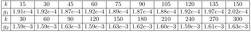
where g3(x) = (1− kxk2)4+(4kxk2+ 1), x∈ [0,1]3. It can be found in Chang et al. (2017) that g1 ∈ HK1 with exponent r = 1/2 in (5) and g2 ∈ HK2 with exponent r > 1/2. We repeat each experiment 40 times and report the average of these experimental results.
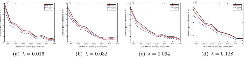
Our numerical results are divided into three parts. In the first part, we study the relation between the generalization ability of BKRR and the regularization parameter to verify our motivation to combine KRR with boosting. In the second part, we validate the empirical behavior of BKRR and its comparison with iterated Tikhonov regularization (ITR). In the last part we show the effectiveness of adaptive stopping rule (16) in practical regression problems.
6.1. Regularization Parameters in BKRR
used to build up a weak learner, this argument then shows that we should select a relatively large λ, larger than some value, so that BKRR with a suitable number of iterations can reach a similar learning performance as KRR. Our first simulation is to verify this argu-ment and show a relation between the generalization ability and regularization parameters in BKRR.
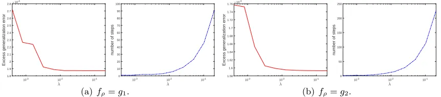
In this simulation, We traverse the regularization parameter λ over the set 0.0002×
{1,2,22, . . . ,210}. For each regularization parameter, we run BKRR until k reaches 150
for fρ = g1 and 300 for fρ = g2, respectively. For each considered k and λ, we estimate the excess generalization error (EGE) E(fD,λ(k))− E(fρ) by 20001 P2000i=1 [fD,λ(k)(x0i)−fρ(x0i)]2,
where{x0i}2000
i=1 are independently drawn from the uniform distribution on the corresponding input space. For each λ, we record the optimal k (selected to be optimal to the test data directly) and the corresponding EGE. Figure 1 reports EGEs and iteration numbers versus regularization parameters. It is shown in Figure 1 that if λ is larger than some value (near 10−2 in this simulation), then BKRR with differentλpossesses similar learning performances provided the number of iterations is appropriately selected. Figure 1 also shows that the more high-level of under-fitting, the more boosting iterations required, which verifies the previous common consensus. All these results show that using KRR to build up a weak learner for boosting is reasonable and the selection of λ does not affect the generalization ability very much.
10-3 10-2 10-1
1.8 1.9 2 2.1 2.2 2.3 2.4 2.5 2.6 2.7 2.8
Excess generalization error
10-4
10-3 10-2 10-1
0 10 20 30 40 50 60 70 80 90 100
number of steps
(a)fρ=g1.
10-3 10-2 10-1
1.58 1.6 1.62 1.64 1.66 1.68 1.7 1.72 1.74 1.76
Excess generalization error
10-3
10-3 10-2 10-1
0 50 100 150 200 250
number of steps
(b) fρ=g2.
Figure 1: Excess generalization errors of BKRR versus regularization parameters. We also plot the iteration number at which the optimal EGEs are achieved.
6.2. Behavior of BKRR
would typically decrease first askincreases from 1 to some number, after which it increases slowly as a function ofk. To be detailed, the increasing curve behaves as a concave function with respect to k, which validates our arguments in Theorem 3 and Theorem 4 that the variance increases with exponentially diminishing terms as k increases. Furthermore, for some largeλ(λ= 0.2048 for example), BKRR shows a rather stable relationship between the generalization performance and iteration numbers. This is consistent with our theoretical findings in Theorem 3 and Theorem 4. We can also see clearly that the iteration numberk
at which EGEs achieve the minimal value would increase as λincreases.
0 50 100 150 10-3
10-2
Excess generalization error
(a)fρ=g1.
0 50 100 150 200 250 300 10-2
Excess generalization error
(b) fρ=g2.
Figure 2: Excess generalization errors versus the number of iterations for different regular-ization parameters. We consider four λ and two regression problems with the regression function beingg1 and g2 in panel (a) and panel (b), respectively.
10-3 10-2 10-1 10-3
Excess generalization error
(a)fρ=g1.
10-3 10-2 10-1 10-2
Excess generalization error
(b) fρ=g2.