The Thirty-Third AAAI Conference on Artificial Intelligence (AAAI-19)
Model-Free IRL Using Maximum Likelihood Estimation
Vinamra Jain,
1Prashant Doshi,
1Bikramjit Banerjee
2 1THINC Lab, Dept. of Computer Science; University of Georgia; Athens, GA 306022School of Computing Sciences & Computer Engineering; University of Southern Mississippi; Hattiesburg, MS 39406 [email protected], [email protected]
Abstract
The problem of learning an expert’s unknown reward func-tion using a limited number of demonstrafunc-tions recorded from the expert’s behavior is investigated in the area of inverse re-inforcement learning (IRL). To gain traction in this challeng-ing and underconstrained problem, IRL methods predomi-nantly represent the reward function of the expert as a lin-ear combination of known features. Most of the existing IRL algorithms either assume the availability of a transition func-tion or provide a complex and inefficient approach to learn it. In this paper, we present a model-free approach to IRL, which casts IRL in the maximum likelihood framework. We present modifications of the model-free Q-learning that re-place its maximization to allow computing the gradient of the Q-function. We use gradient ascent to update the feature weights to maximize the likelihood of expert’s trajectories. We demonstrate on two problem domains that our approach improves the likelihood compared to previous methods.
1
Introduction
Inverse reinforcement learning (IRL) (Russell 1998) is the problem of ascertaining an agent’s preferences from obser-vations of its behavior on a task. It inverts RL with its focus on learning the reward function given information about op-timal action trajectories. IRL lends itself naturally to a robot learning the task from demonstrations by a human teacher (often called the expert) in controlled environments, and therefore finds application in robot learning from demonstra-tion (Argall et al. 2009), imitademonstra-tion learning (Osa et al. 2018), and forming ad hoc collaborations (Trivedi and Doshi 2018). Key model assumptions of popular IRL methods are that the expert’s stochastic transition function is fully known to the learner as in IRL for apprenticeship learning (Abbeel and Ng 2004) and in Bayesian IRL (Ramachandran 2007). Al-ternately, the transition function is effectively deterministic and thus is easily approximated from the observed trajecto-ries as in entropy maximization (Ziebart et al. 2008) with the assumption that transition randomness has a limited ef-fect on the final behavior. The prior knowledge requirement is often difficult to satisfy in practice, for example, in sce-narios where environmental noise is not random and it influ-ences transitions significantly. An example of this is learning Copyright c2019, Association for the Advancement of Artificial Intelligence (www.aaai.org). All rights reserved.
the driving styles of cars in the merging lane of a congested freeway; cars adjacent to the merging lane add noise. On the other hand, assuming that any transition error is incon-sequential is a strong imposition in the context of robots.
In this paper, we introduce novel model-free algorithms to generalize IRL to problem domains where the transition function is not available. A previous method for model-free IRL (Boularias, Kober, and Peters 2011) casts the problem as one of relative entropy optimization while using impor-tance sampling to avoid using the model. A more recent method (Uchibe 2018) casts IRL as a problem of estimat-ing the density ratio between expert state transitions and a baseline one, and shows how this is related to the reward function in linearly solvable MDPs where the state transition probability is optimized. Both of these methods assume the availability of a secondary set of (non-expert) trajectories. In stark contrast, our approach does not require this secondary set of trajectories. We build on the model-based maximum likelihood IRL (MLIRL) (VRoman 2014) to remove its de-pendency on the transition function. Our method replaces the traditional Bellman update in MLIRL with two ways of performing model-free Q-learning that is modified to be dif-ferentiable. The first modification is to replace themax op-erator in the update with an averaging opop-erator. The second modification replaces the max operator with a Boltzmann-weighted mean. As we show, the search for the most likely reward function can now be guided by the gradient of the likelihood function for the current feature weights.
in the context of freeway merging. In all of these evalua-tions, our methods meet and often exceed the performance of MLIRL, while easily improving on the performance of relative-entropy IRL. Between the two modifications, the av-eraging estimation is significantly better. These results make the maximum-likelihood IRL with the Q-averaging estima-tion as the new frontline method for model-free IRL.
2
Background
In this section, we briefly review the fundamentals of IRL and the maximum likelihood estimation approach to IRL.
2.1
Inverse Reinforcement Learning
Informally, IRL refers to both the problem and method by which an agent learns preferences of another agent that ex-plain the latter’s observed behavior (Russell 1998). Usually considered an “expert” in the task that it is performing, the observed agent, sayI, is modeled as executing the optimal policy of a standard MDP defined ashSI, AI, TI, RIi. The learning agent is assumed to perfectly know the parameters of the MDP except the reward function. Consequently, the learner’s task may be viewed as finding a reward function under which the expert’s observed behavior is optimal.
This problem in general is ill-posed because for any given behavior there are infinitely-many reward functions which align with the behavior. Abbeel and Ng (2004) present an al-gorithm that allows the expertIto provide task demonstra-tions instead of its policy. The reward function is modeled as a linear combination ofKbinary features,φ:SI×AI → {0,1}, each of which maps a state from the set of statesSI
and an action from the set ofI’s actionsAI to either a 0 or
1. Note that non-binary feature functions can always be con-verted into binary feature functions although there will be more of them. Throughout this paper, we assume that these features are known to, or selected by, the learner. The re-ward function for expert I is then defined as RI(s, a) =
PK
k=1θk·φk(s, a), whereθk are theweights. The learner’s
task is reduced to finding a vector of weights that complete the reward function, and subsequently the MDP such that the demonstrated behavior is optimal.
To assist in finding the weights, feature expectations are calculated for the expert’s demonstration and com-pared to those of possible trajectories (Ziebart et al. 2008). A demonstration is provided as one or more trajecto-ries, which are a sequence of length-T state-action pairs,
(hs, ai1,hs, ai2, . . .hs, aiT), corresponding to an
observa-tion of the expert’s behavior across T time steps. Feature expectations of the expert are averages over all observed tra-jectories,φˆk = |X1|
P
x∈X
P
hs,ai∈xφk(s, a), wherexis a
trajectory in the set of all observed trajectories,X.
Given a set of reward weights, the expert’s MDP is com-pleted and solved optimally to produceπI∗. The difference
ˆ
φ −φπ∗I provides a gradient with respect to the reward
weights for a numerical solver. To resolve the degeneracy of this problem, Abbeel and Ng (2004) maximize the mar-gin between the value of the optimal policy and the next best policy. The resulting program may be solved with a quadratic program solver such as a support vector machine.
2.2
MLE for Model-based IRL
Babes-VRoman et al. (2014) showed how IRL could be for-mulated as a maximum likelihood estimation (MLE) prob-lem.
θ= arg max
θ∈Θ L(θ)
whereL(θ)is the log-likelihood of the demonstration tra-jectories inX. In other words,
L(θ) = logP r(X;θ) (1)
As the trajectories in X are conditionally independent of each other givenθ, we can decomposeP r(X;θ)as:
P(X;θ) = Y x∈X
P(x;θ) (2)
Becausexdenotes a trajectory as shown in Section 2.1, we may further decompose Eq. 2 as:
P r(X;θ) =Y x∈X
P r(s1)P r(a1|s1;θ)
T−1
Y
i=1
P r(si+1|si, ai)
×P r(ai+1|si+1;θ)
. (3)
The termP r(ai+1|si+1;θ)is given by the agent’s policy
pa-rameterized byθ, andP r(si+1|si, ai)is given by the
transi-tion functransi-tion. Therefore,
P r(X;θ) =Y x∈X
P r(s1)πθ(s1, a1)
T−1
Y
i=1
T(si, ai, si+1)
×πθ(si+1, ai+1)
.
Taking log on both sides we get the log likelihood as,
L(θ) =X x∈X
log P r(s1) + T−1
X
i=0
log πθ(si+1, ai+1)
+ T−1
X
i=1
log T(si, ai, si+1)
!
. (4)
The transition function in the log likelihood above is usually given. Therefore, it is common practice to exclude it from the computation while comparing the performance of vari-ous methods (Ramachandran 2007; VRoman 2014).
L(θ) =X x∈X
log P r(s1) + T−1
X
i=0
log πθ(si+1, ai+1) !
.
(5) The policy is commonly modeled using the parameter-ized Boltzmann exploration (Ramachandran 2007; VRoman 2014) as follows,
πθ(s, a) =
eβ Qθ(s,a)
P
a0∈A
Ie
β Qθ(s,a0) =
eβ Qθ(s,a) Zθ(s)
. (6)
function becomes,
Qθ(s, a) =Rθ(s, a) +γ X
s0∈S
I
T(s, a, s0)
× X
a0∈AI
Qθ(s0, a0)πθ(s0, a0) (7)
whereπθ(s0, a0)is as defined in Eq. 6.
To obtain the MLE, we may partially differentiate the log likelihood of Eq. 5:
∂L(θ) ∂θ =
X
x∈X T
X
i=1
1 πθ(si, ai)
∂πθ(si, ai)
∂θ (8)
In the context of Eq. 6, differentiating the policy above in-volves differentiating the Q-function w.r.t.θ. Although the derivative of the Q-function requires differentiating the pol-icy in turn, Babes-VRoman et al. (VRoman 2014) show how this recursive differentiation may be performed and the fea-ture function weights are updated using the standard gradi-ent descgradi-ent until the weights all converge. Notice that the computation of the Q-function involves the transition func-tion of the expertI.Consequently, the approach given by Babes-VRoman et al. is a model-based MLE for IRL.
3
Model-Free MLE for IRL
We are motivated to study model-free IRL because it relaxes a debilitating prior knowledge requirement by most IRL methods. Specifically, they assume that the learner knows the dynamics of the expert as modeled by its stochastic tran-sition function as in apprenticeship learning (Abbeel and Ng 2004) and in Bayesian IRL (Ramachandran 2007). Alter-nately, the transition function is assumed to be effectively deterministic and thus is easily approximated from the ob-served trajectories as in entropy maximization (Ziebart et al. 2008) with the assumption that transition randomness has a limited effect on the final behavior. The prior knowledge requirement is often difficult to satisfy in practice, for ex-ample, in scenarios that are not cooperative. Alternately, the supposed impotency of transition errors is a strong assump-tion in the context of robots possessing noisy actuators.
Two observations enable us to adapt the MLE of Sec-tion 2.2 for model-free IRL. First, notice that the right-hand side of the gradient of the log likelihood in Eq. 5 does not involve the transition function. Second, if we replace the Q-function computation in Eq. 7 with a way of computing it that does not involve the transition function, then the gra-dient can be entirely computed without knowledge of the transition function.
We begin by presenting a method to estimate the Q-value without knowledge of the transition function.
3.1
Differentiable learning
A straightforward model-free estimation of the expert’s
Qθ(s, a)is to use Watkin’s off-policy Q-learning (Watkins
and Dayan 1992).
Qθ(s, a)← (1−α)Qθ(s, a) +α Rθ(s, a)+
γ max a0∈A
I
Qθ(s0, a0))
whereαis the learning schedule,γis the discount factor,s0
is the next state in the trajectoryx, andRθ(s, a)is the reward
for taking actionain state s. Recall that the reward func-tion is defined asRθ(s, a) = P
K
k=1θk φk(s, a).However,
the presence of the maxoperator in the estimation above makes the Q-function discontinuous and therefore not dif-ferentiable (Asadi and Littman 2017).
Consequently, as a first step, we seek a simple modifica-tion of the Q-learning equamodifica-tion to make it differentiable. We propose two estimations of the Q-function, first of which re-places the max operator with an averaging operator.
Qθ(s, a)←(1−α)Qθ(s, a) +α Rθ(s, a)+
γ
P
a0∈A
IQθ(s
0, a0)
|AI|
(9)
Notice that the averaging operation simply replaces the max-imal Q-value for the next states0with the Q-value averaged over all expert’s actions for the next state. We refer to this version of Q-learning asQ-averaging. This use of the av-eraging operation for IRL is novel to the best of our knowl-edge.
The second estimation replaces the max operator with the Boltzmann-weighted mean as given below:
Qθ(s, a)←(1−α)Qθ(s, a) +α Rθ(s, a)+
γ X
a0∈A
I
πθ(s0, a0)Qθ(s0, a0) (10)
Here, πθ(s0, a0) is the Boltzmann softmax as defined in
Eq. 6. We refer to this version of Q-learning asQ-softmax. For both these Q-learning methods, we will continue to use the Boltzmann policy for the action distribution. This introduces a discrepancy between how the Q-value is esti-mated inQ-averaging– essentially selecting one of the ex-pert actions at s0 at random – and the action distribution. However, not all is lost with this approximation. In addi-tion to being easily differentiable, theQ-averagingupdate is a non-expansion given fixed θ ensuring convergence to a unique fixed point (Asadi and Littman 2017). As such, it serves as a useful method. In comparison,Q-softmaxis dif-ferentiable and approximates the traditional “max” operator for selecting an action ats0 asβ → ∞. However, it lacks the non-expansion property and therefore may not always converge.1
3.2
Gradient Computation
Our approach is to obtain the gradient vector of the log like-lihood, which is defined as:
∇L(θ) =
∂L(θ)
∂θ1
,∂L(θ) ∂θ2
, . . . ,∂L(θ) ∂θk
1
We may then use the appropriate component of the gradi-ent vector to update the parametersθ as a step of gradient ascent.
∀i, θtk+1=θkt+αt∇Lk(θ)
where,αtis the dynamic step size in thetthiteration and ∇Lk(θ)denotes the component of the gradient correspond-ing to the differentiation byθk.
The derivative of the log likelihood in Eq. 8 requires com-puting the gradient of the policy. This is obtained as,
∂πθ(si, ai)
∂θ =
1 Z2
θ(s)
Zθ(s)β eβ Qθ(s
i,ai)∂Qθ(si, ai)
∂θ
−eβ Qθ(si,ai) ∂Zθ(s) ∂θ
. (11)
Q-averaging The above requires the gradient of the Q-function, whose computation proceeds as follows for Q-averaging. Equation 9 is iterated until (near-)convergence. For thetthiteration, we may write it as:
Qθt(s, a) = (1−α)Qθt−1(s, a) +α Rθ(s, a)+
γ |AI|
X
a0
Qtθ−1(s0, a0)
(12)
and its gradient becomes,
∂ ∂θkQ
t
θ(s, a) = (1−α)
∂ ∂θkQ
t−1
θ (s, a) +α φk(s, a)+
γ |AI|
X
a0
∂ ∂θkQ
t−1
θ (s
0, a0)
(13)
As the Q-function at the first time step is the reward func-tion, we get,
∂ ∂θkQ
1
θ(s, a) =
∂
∂θkRθ(s, a) =φk(s, a) (14)
Recall that Q-averaging is a non-expansion given θ and differentiable. Consequently, iterating over Eq. 13 with Eq. 14 as the base case will cause the gradient to converge to a fixed point. As such, the gradient of the model-free Q-function is available to us.
Next, we need the gradient ofZθw.r.t.θk, which uses the
converged gradient of the Q-function obtained before.
∂Zθ(s)
∂θk =β
X
a∈AI
eβ Qθ(s,a) ∂ Qθ(s, a) ∂θk
=β X
a∈AI
eβ Qθ(s,a)
(1−α)∂Qθ(s, a)
∂θk +
α φk(s, a) + γ |AI|
X
a0
∂Qθ(s0, a0)
∂θk
We summarize the method for model-free IRL using Q-averagingin Algorithm 1. We initialize the feature weight vector and the Q-table with random values and zeroes re-spectively, and compute the initial policy (lines 1-4). For
Algorithm 1Model-free ML IRL usingQ-averaging Require: MDP\{R, T}: hS, AI, γi, Features
Φ :{φ1, φ2, ..., φK}, TrajectoriesX:(x1, x2, . . . , xN), α,αn,
1: Initialize randomlyθ:hθ1, θ2, . . . , θki
2: Initialize local variablesL0←0,n←0,t←0
3: InitializeQθ(s, a)←0for alls∈S,a∈AI
4: Initialize stochastic policy using Eq. 6 5: repeat
6: n←n+ 1
7: L←L0
8: Rθ(s, a) =P
K
k=1θk φk(s, a)
9: repeat
10: t←t+ 1
11: UpdateQtθ(s, a)(Eq. 12) for all(s, a)using Boltz-mann exploration
12: Update∂Qtθ(s,a)
∂θk using Eq. 13 for all(s, a)andθk
13: Use Eq. 6 and updated Q-values to update policy 14: until|Qt
θ(s, a)−Q
t−1
θ (s, a)|< (1−γ)/γ
15: Q∗θ(s, a)←Qt
θ(s, a)for all(s, a)
16: πθ(s, a)← e
βQ∗θ(s,a) P
a0e
βQ∗θ(s,a0) for all(s, a)
17: Evaluate likelihoodL(θ)using Eq. 5 18: Obtain∇Lk(θ)(Eq. 8) using
∂Qtθ
∂θk in Eq. 11
19: L0←L(θ)
20: for allθk∈θdo
21: θk←θk+αn∇Lk(θ)
22: δ=|L0−L| 23: untilδ < (1−γ)/γ
24: return θ
the current θ, we obtain the nearly converged Q-values and its gradient in an iterative manner. The model-free Q-averaginguses the Boltzmann policy (kept updated) for ex-ploration (lines 9-14). These are then utilized to obtain the current log likelihood for the expert’s trajectories and its gra-dient. Lines 20-22 perform gradient ascent to update the fea-ture weights, and these steps are repeated until approximate convergence.
Q-softmax Let us proceed in a similar manner as in Q-averaging, and write out the iterative version of the Q-function.
Qθt(s, a)←(1−α)Qθt−1(s, a) +α Rθ(s, a)+
γ X
a0∈A
I
πtθ−1(s0, a0)Qtθ−1(s0, a0)
(15)
where for any iteration t the probability πt
θ(s, a) is
ob-tained from thetthiteration of the Q-function,πt
θ(s, a) =
eβ Qtθ(s,a)
P
a∈AIe
β Qtθ(s,a) =
eβ Qtθ(s,a) Zt
θ(s)
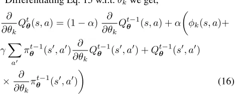
Differentiating Eq. 15 w.r.t.θkwe get,
∂ ∂θk
Qtθ(s, a) = (1−α) ∂ ∂θk
Qtθ−1(s, a) +α
φk(s, a)+
γX
a0
πθt−1(s0, a0) ∂ ∂θkQ
t−1
θ (s
0, a0) +Qt−1
θ (s
0, a0)
× ∂
∂θkπ t−1
θ (s
0, a0)
(16)
Notice that Eq. 16 also involves the gradient of the policy in contrast to the gradient ofQ-averaging. This is obtained analogously to Eq. 11 with the difference thatQθ(s, a)and
its derivative is replaced withQtθ−1(s, a)and its derivative, respectively, both of which are available from the previ-ous iteration. WithQ-softmaxnot guaranteed to be a non-expansion, its gradient may not be a non-expansion either in some cases. Finally, we obtain the gradient ofZt
θas,
∂Zt
θ(s)
∂θk
=β X
a∈AI
eβ Qtθ(s,a) ∂ Q t
θ(s, a)
∂θk
where∂ Qtθ(s,a)
∂θk is computed as given in Eq. 16.
The algorithm for model-free IRL with MLE using Q-softmax is analogous to Algorithm 1 with just a few changes. In particular, the Q-value in line 11 is updated us-ing Eq. 15 and its gradient in the next line is computed usus-ing Eq. 16. The remaining steps of the algorithm including the likelihood computation and the iterative update of feature weights remain unchanged.
4
Experiments
We evaluated our model-free IRL algorithm using two ap-plication domains. Multiple experiments were performed on two domains: the grid world domain, a small toy lem, and the freeway merging domain, a real-world prob-lem with a considerably larger state space than the first. We also compared our results with the model-based MLIRL approach and another model-free approach, relative en-tropy IRL (REIRL). We used Monica Babes-VRoman’s code for MLIRL, and REIRL code from https://github.com/ aravindsiv/irl-lab. Our code for both presented methods is also publicly available at https://github.com/RAILUSM/ Model-free-IRL.
4.1
Gridworld Domain
Our first domain is a simple grid of size5×5. An agent can navigate this domain using 4 directional movements. Fig-ure 1 depicts the graphical user interface for the grid world environment. The gray colored circle is the agent. The five different color grids signify the unique location features.
The MDP model for the grid world environment includes 25 states, 4 actions, and the discount factor of 0.99. The task is to reach the nearest corner (goal) cell from any non-blue starting location, while avoiding the blue cells. We used two variants of this domain—one with no transition noise, and another where the agent has a 10% chance of slipping later-ally relative to the intended direction of motion. We used the Boltzmann temperature (β) as 0.01 for all methods.
Figure 1: The graphical user interface for grid world envi-ronment. The gray circle is the agent exploring the 5×5
grid. Each different color in the grid represents a distinct (Boolean) feature of the state. The agent tries to learn the cost associated with each color using the expert’s trajecto-ries.
We recorded 20 trajectories in each variant, by moving the agent across the grid following an optimal policy for the above tasks. We then removed any repeated trajecto-ries, leading to a set of 12 distinct expert trajectories in 0-noise variant, and 14 distinct expert trajectories in 10%-noise variant. These trajectories were then used by the agent to learn the reward weights associated with each grid-color (feature). The weights were initialized to random values in
[−1,1] for all methods. Accurate transition matrices–with or without noise–were additionally available to the model based method (MLIRL). While MLIRL and our methods are based on the log-likelihood of data, REIRL does not use this metric, and instead runs for a given number of iterations. We allowed it5×105iterations in the no-noise variant, and106
Method Learned feature weights (feature 5 is blue) Final
θ1 θ2 θ3 θ4 θ5 log-likelihood
MLIRL 43.04±14.83 33.31±11.35 54.23±18.23 53.93±18.00 −49.09±16.80 −36.50±3.12
Q-Avg 152.33±60.81 92.06±36.91 1526.06±608.96 151.51±60.49 0.03±0.56 −29.25±6.59 Q-SM 17.92±14.09 11.96±9.15 109.88±84.96 17.87±14.07 0.02±0.60 −40.39±4.15
REIRL 0.87±0.00 28.27±0.60 40.43±0.58 44.62±0.55 −3.10±0.05 −43.58±0.03
Table 1: Comparison of learned feature weights and corresponding final log-likelihood values of trajectories for grid world domain with no transition noise, from various algorithms.
Method Learned feature weights (feature 5 is blue) Final
θ1 θ2 θ3 θ4 θ5 log-likelihood
MLIRL 94.00±31.88 86.91±29.56 93.26±31.67 95.35±32.11 −71.57±23.78 −45.05±9.07
Q-Avg 227.72±1.41 89.83±0.68 157.59±1.18 3368.95±0.24 151.43±0.67 −40.49±0.04 Q-SM 30.37±5.22 10.98±1.69 18.40±2.91 225.20±0.21 11.33±0.80 −57.35±0.30
REIRL 0.58±0.09 0.13±0.05 1.96±0.46 0.31±0.06 −0.50±0.40 −72.11±0.01
Table 2: Comparison of learned feature weights and corresponding final log-likelihood values of trajectories for grid world domain with 10% transition noise, from various algorithms.
the no-noise variant (Table 1). With transition noise, how-ever, the blue feature sometimes appears in the expert tra-jectories due to slippage, but without a true transition matrix or baseline trajectories our methods have no way to real-ize that this feature is undesirable to the expert. Hence we see higher weights associated with this feature for both Q-averagingandQ-softmaxin Table 2. Notwithstanding this, the final log-likelihoods of our methods are competitive, in particular,Q-averagingachieves the highest log-likelihood in both cases. The relatively large variances for some indi-cate that different trials converged to different local optima. This is a consequence of the termination criterion (line 23 of Algorithm 1) which was also applied to MLIRL, and this may explain why despite being model-based it failed to find solutions with higher log-likelihoods on the average.
A Wilcoxon signed rank test of significance between the sets of final log-likelihoods of different methods compared to MLIRL found that for the no-noise case, theQ-averaging
method achieves significantly higher log-likelihoods than MLIRL at the 99% confidence level (p-value=0.00194), while MLIRL achieves significantly higher log-likelihoods compared to Q-softmax and REIRL (p-value 0 in both cases). In the 10% noise gridworld, the same relative ad-vantages hold with p-values 0, 0, and 0 respectively.
Instead of a comparison of precise run times (because the methods were implemented in different programming languages), we note that all methods ran in a comparable amount of time, each under 15 minutes per trial on a Linux workstation with Intel core i7 CPU each core is 3.6GHz and 16GB of main memory.
4.2
Freeway Merging Domain
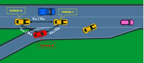
The freeway merging domain is a real-world problem faced by autonomous vehicles in making decisions about when to merge, keeping in consideration the stochastic behavior of human drivers on the freeway. Solving the freeway merg-ing problem requires modelmerg-ing the relevant traffic. Here, we model this problem using a sufficient A-B-C model as shown
in Fig. 2. Vehicle in role B is an autonomous vehicle that is about to merge onto the freeway. A is the vehicle on right-most lane of the freeway but relatively behind B. C is also the vehicle on rightmost lane of the freeway but relatively ahead of B. The problem is that vehicle B must merge between A and C but the preferences of A’s driver about allowing B to merge ahead are not known. The objective of IRL in this context is to model the preferences of A’s driving model as it detects B.
Figure 2: Detailed A-B-C model representing the freeway merging problem. B is an autonomous vehicle about to merge onto the freeway. Relative variables like velocity and distance between any two vehicles play crucial roles in defining the state of vehicle in role A.
adjacent to the freeway to record vehicle passing through over approximately 500 meters (1,640 feet) in length. The study included all 6 freeway lanes and an additional on-ramp merging onto the freeway. The collected dataset is well doc-umented with necessary meta-data. Out of the 260 trajecto-ries in the full dataset that encompasses a wide variety of driving preferences, we isolated 12 trajectories where A ex-hibited risky behavior, accelerating frequently. This experi-ment is based on these 12 trajectories.
We define the state space using the following 5 state vari-ables:
1. dAC: Distance between vehicles A and C (inf t.) 2. dAB: Distance between vehicles A and B (inf t.) 3. vAC: Velocity of A relative to C (inf t./sec)
4. vAB: Velocity of A relative to B (inf t./sec)
5. Vehicle type of vehicle B (truck or not).
We discretized the first 4 state variables into 5 intervals and the fifth variable is binary in nature. This yields 1,250 states of vehicle A.
The instantaneous acceleration values are modeled as actions of the driver. We discretized the acceleration (in
f t./sec2.) into five intervals and named them as the follow-ing actions:
1. High Brake:−11.20≤acc≤ −4.80
2. Low Brake:−4.79≤acc≤ −0.60
3. Zero Acceleration:−0.59≤acc≤0.59
4. Low Acceleration:0.60≤acc≤4.79
5. High Acceleration:4.80≤acc≤11.2
We accounted for 3 binary features in the reward func-tion. Any feature is considered active with the value 1 and inactive when the value is 0.
Safe (φ1): This feature is inactive only whendAC <35f t.
andacc≥0.6f t./sec2, i.e. distance from the preceding
vehicle is less than 35 ft and the vehicle is accelerating. This feature signifies the preference of being safe when active.
Time to travel (φ2): This feature is active when acc >
−0.6 f t./sec2, i.e. either the vehicle is accelerating or
moving with a constant speed. This feature signifies the importance of time to reach the destination.
Ahead of Truck (φ3): This feature is active when the
vehi-cle B is a truck andacc≥0.6f t./sec2, i.e., A accelerates
when B is a truck to get ahead of it.
Below is the summarized description of the experimental setup.
• M DP :hS, A, γi=h1250,5,0.99i;
• FeaturesΦ ={φ1, φ2, φ3};
• T ={ζ1, ζ2, ..., ζ12}, i.e. set of 12 expert’s trajectory
ex-hibiting risky behavior from the NGSIM dataset;
• Boltzmann temperature,β = 0.01;
• Learning rate for Q-averaging and Q-softmax, α = 0.01.
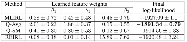
Table 3 shows the learned feature weights and corre-sponding final log-likelihood values of trajectories using our model-free IRL approach as well as the existing baselines MLIRL and REIRL, based on 10 independent trials for each setting. MLIRL requires the transition model, which we es-timated by relative frequency of transition counts from the trajectories. For states not seen in the trajectories, we ap-plied the mid-point of action ranges to the midpoint of state feature ranges to estimate the next states using standard dy-namical equations. Although this is a reasonable model, the result is unlikely to be an accurate transition model for a domain as complex as NGSIM, and this highlights a ma-jor limitation of model-based approaches. For REIRL, we prolonged shorter trajectories by assuming constant veloc-ity motion for A, B, and C beyond the last frame. We also selected a subset of trajectories randomly from the full set (of 260 trajectories) to serve as the baseline trajectories for REIRL. Once again, we see from Table 3 thatQ-Averaging
achieves the best log-likelihood, while this time MLIRL achieves the worst, perhaps because the estimated transition model is a poor approximation in this domain. In particular, MLIRL terminated early, in less than 25 iterations in all tri-als, confirming the unsuitability of a model-based approach for a complex domain where just the trajectory data is avail-able. The log-likelihoods in Table 3 indicate performance improvement in the order MLIRL<REIRL<Q-softmax <Q-averaging, with the Wilcoxon signed rank tests being significant at the 99% level (p-values across successive pairs being 0.00694, 0.00512, 0.00512). While the selection cri-terion for the 12 trajectories, viz., vehicle A speeding often, may indicate that the weight of the second feature (i.e.,θ2)
should be the highest, that is not the case forQ-averaging
and REIRL. However, the intuition is essentially correct, be-cause the trials whereθ2ended up higher forQ-averaging
also had a slightly higher log-likelihood (≈ −1890). Unfor-tunately, only 40% of the trials converged to this solution. Once again the methods had comparable runtimes (except MLIRL which exited early with poor solutions) of about one hour per trial.
The overall results in Table 3 indicate a few interesting conclusions about the trajectories themselves. Even though the trajctories were selected based on what appeared to be risky driving behavior, the methods reach the conclusion that vehicle A still prefers to maintain safety. Also, contrary to the other methods, REIRL came to the conclusion that vehi-cle A strongly prefers to get ahead of B when the latter is a truck. However, given that both our methods achieve higher log-likelihoods with low values ofθ3, we must conclude that
the trajectories display insufficient evidence of this behavior.
5
Conclusion and Future work
log-Method Learned feature weights Final
θ1 θ2 θ3 log-likelihood
MLIRL 0.28±0.72 0.42±0.48 0.45±0.76 −1927.09±1.1
Q-Avg 2.01±0.23 1.86±0.37 0.15±0.55 −1891.34±0.79 Q-SM 0.41±0.30 0.80±0.53 −0.12±0.67 −1914.56±1.38
REIRL 0.08±0.18 0.01±0.14 15.89±7.62 −1920.48±3.24
Table 3: Comparison of learned feature weights and corresponding final log-likelihood values of NGSIM trajectories, from various algorithms.
likelihood compared to both an existing model-based and a model-free method. Furthermore, the experiment on a real-world complex problem involving freeway merging, high-lights the considerable limitation of model-based MLIRL. Thus our experimental findings positionQ-averagingas the new state-of-the-art for model-free IRL.
It may appear surprising thatQ-averagingis able to per-form so well despite involving no optimization within the Q-update rule itself. Note however, that it simply gives a plausible value estimate of the policy in the current itera-tion, while the real search is in the space of feature weights, where gradient ascent provides the needed optimization in IRL. During algorithm design, we expectedQ-softmaxto perform better since it is closer to the Bellman operator for high values ofβ, and it is instructive to inspect why it did not. We found that high values of β leads to exponential blow-up in the gradient values (due to the presence of ex-ponential terms in equation 11) and this forced us to use smallerβ values in the experiments. Note that this problem appears with the MLIRL method as well. Smallerβactually makes the Q-values ofQ-averaging andQ-softmax(i.e., equations 12 and 15) to be rather similar; however their gra-dients (equations 13 and 16) are quite different. The net ef-fect on the learning outcome seems to be that theQ-softmax
gradients tend to keep the feature weights (θ) closer to each other, compared toθ ofQ-averagingwhich can be vastly different (see Tables 1– 3). It appears to effectively become a kind of constraint forQ-softmax, which might explain why it was unable to reach better log-likelihoods.
Future work may include implementing our approach with other optimization techniques which do not require dif-ferentiating the likelihood function. This will allow the use of conventional Q-learning with the “max” operator. Our current approach is limited to a single expert, therefore an-other avenue would be to address multiple experts. Modeling of a multi-agent environment and their interaction with other experts in the environment might lead to better understand-ing of their behavior.
6
Acknowledgment
We thank Tomoki Nishi of Toyota Research Institute of North America and TCRDL for many helpful discussions and insights into the freeway merge domain. We thank Mon-ica Babes-VRoman for her MLIRL implementation which was used to generate baseline results in this paper. We also thank the anonymous reviewers for constructive comments and suggestions. This work was supported in part by a
re-search contract with the Toyota Rere-search Institute of North America (TRI-NA), and by National Science Foundation grants IIS-1830421 and IIS-1526813.
References
Abbeel, P., and Ng, A. 2004. Apprenticeship learning via inverse reinforcement learning. InICML, 1.
Alexiadis, V.; Colyar, J.; and Halkias, J. 2007. A model endeavor. Public Roads70(4).
Argall, B. D.; Chernova, S.; Veloso, M.; and Browning, B. 2009. A survey of robot learning from demonstration. Robotics and Autonomous Systems57(5):469–483.
Asadi, K., and Littman, M. 2017. An alternative softmax operator for reinforcement learning. InInternational Con-ference on Machine Learning (ICML).
Boularias, A.; Kober, J.; and Peters, J. 2011. Relative en-tropy inverse reinforcement learning. InAISTATS, 182–189. Kuderer, M.; Gulati, S.; and Burgard, W. 2015. Learning driving styles for autonomous vehicles from demonstration. InIEEE International Conference on Robotics and Automa-tion (ICRA), 2641–2646.
Osa, T.; Pajarinen, J.; Neumann, G.; Bagnell, J. A.; Abbeel, P.; and Peters, J. 2018. An algorithmic perspective on imi-tation learning. Foundations and Trendsrin Robotics 7(1-2):1–179.
Ramachandran, D. 2007. Bayesian inverse reinforcement learning. InIJCAI, 2586–2591.
Russell, S. 1998. Learning agents for uncertain environ-ments (extended abstract). InEleventh Annual Conference on Computational Learning Theory, 101–103.
Trivedi, M., and Doshi, P. 2018. Inverse learning of robot behavior for collaborative planning. InIROS, 6.
Uchibe, E. 2018. Model-free deep inverse reinforcement learning by logistic regression. Neural Processing Letters 47(3):891–905.
VRoman, M. C. 2014. Maximum Likelihood Inverse Rein-forcement Learning. Ph.D. Dissertation, Rutgers University. Watkins, C., and Dayan, P. 1992. Q-learning. Machine Learning Journal8(3/4).