Study on the Analysis and Optimization of Brake Disc: A Review

(1)

255 Copyright © 2016. Vandana Publications. All Rights Reserved.

Volume-6, Issue-6, November-December 2016

International Journal of Engineering and Management Research

Page Number: 255-260

Classification Analysis to Predict a Closing Price Condition of the Stock of

UNVR using the Gaussian Copula Model

Aulia Ikhsan1, Bagus Sartono2, Anik Djuraidah3

1,2,3_{Department of Statistics, Bogor Agricultural University, INDONESIA}

ABSTRACT

Copula introduced first by Abe Sklar at 1959 in Sklar’s Theorem that represented bond or tie. Copula Modeling mostly used in multivariate analysis as alternative if multivariate normal distribution assumption not fulfilled. In this research, will do classification analysis based on Gaussian Copula Model to classify or to predict increase or decrease the stock price of PT Unilever Indonesia (UNVR) based on increase or decrease of LQ-45 Index (LQ45), Consumer Good Index (KMSI), Jakarta Composite Index (IHSG), and stock price of PT Wismilak Inti Makmur at Indonesian Stock Exchange during 111 days of exchange (January 5, 2016 – June 14, 2016). Prediction process do with simulation data that built using couple information in research data that one of them is distribution for each variable. As for the results achieved are the value of the biggest increase and decrease stock price UNVR successively is 0.0529 and -0.0473. The identified distribution with estimate parameter for each variable is UNVR ~ Bernoulli (0.46), LQ45 ~ Normal (0.000370, 0.009267), KMSI ~ Logistic (0.000841, 0.006491), IHSG ~ Normal (0.000370, 0.009267), and WIIM ~ Cauchy (-0.000735, 0.008259). While the result of prediction has prediction accuracy rate and error prediction rate successively is 68.47% and 31.53%.

Keywords— Classification Analysis, Gaussian Copula, Sklar’s Theorem, UNVR

I. INTRODUCTION

At multivariate statistics research for data in Finance and Climatology, often got variables from data that used in research not follow multivariate normal distribution. While in multivariate analysis many methods that assuming that data will analyzed must follow multivariate normal distribution. But if the assumption not fulfilled, then there are several multivariate distribution can be used. The several distributions are bivariate gamma distribution1 and bivariate exponential distribution2. But several multivariate probability distribution still have

several limitation, there are composer univariate distribution must have same distribution and multivariate distribution density function that usually have complex structure3. Many research had been done to handle this problem, one of them is copula model research.

Copula first introduced by Abe Sklar at 1959 and bring forth Sklar’s Theorem as the base of copula theory. Copula is mean bond or tie that intended to explain about several random variables that “boned” became one to form a multivariate distribution function. The advantages of copula are invariant towards random variable transformation4, not strict towards distribution assumption for random variable copula composer, and can be used for many random variables. Several research from many fields had been used copula model, that is in climatology research5,6. and finance7,8,9. So copula model can be use as multivariate distribution alternative along with multivariate analysis.

Multivariate analysis has many methods based on analysis purpose. One of them is classification analysis, analysis that used to classify several observations or several objects that have several attribute to several groups based on certain classification rules. Several research related to classification analysis had been done with copula model10,11. There for this research will predict closing price condition of PT Unilever Indonesia with classification analysis using Gaussian copula model.

II. METHODOLOGY

(2)

256 Copyright © 2016. Vandana Publications. All Rights Reserved.

( , , , ). Each variable observed during 111 days

exchange started from January 5, 2016 until June 14, 2016. Then the data can be called as training data. R software with package fitdistrplus, MASS, and fields is used to help data analysis process. As for data analysis step is already summarized in figure 1.

Y: Closing price category of PT Unilever Indonesia (UNVR) based on return (0=Not Decrease, 1=Decrease) X0: Closing price return of PT Unilever Indonesia (UNVR)

X1: Opening index return of LQ-45 Index (LQ45)

X2:Opening index return of Consumer Good Index (KMSI)

X3:Opening index return of Jakarta Composite Index

(IHSG)

X4:Closing price return of PT Wismilak Inti Makmur

(WIIM)

Figure 1: Flowchart of Data Analysis

III. PRIOR APPROACH

Let

is an distribution function with the

dimension with margins

, then there will a copula for entire in

̅

as:

(

)

(

)

(

)

(

))

Let entire

is continuous, then is unique. Otherwise, determined in unique way at

. Oppositely, let is copula with the dimension

and

are distribution function, then

function defined on equation

2.1 is a distribution function with dimension

with

margin functions

12_.

IV. OUR APPROACH

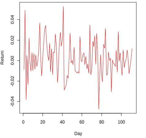
Return movement closing stock price PT Unilever Indonesia can be saw at Figure 2. Based on figure 2, obtainable information that closing stock price PT Unilever Indonesia during January 2016 until June 2016 had fluctuating movement around 0 with highest return closing stock price is 0.05286 that happen at march 2, 2016 and lowest return closing stock price is -0.04734 that happen at April 25, 2016.

Figure 2: Return Movement of UNVR

To make Gaussian copula model, distribution identification from each marginal composition distribution must be made. Refer to the value on Table I, can be seen that each variable predictor have skewness value and kurtosis that different between one and the other. Based on this information, distribution identification for each variable predictor must be made because each variable predictor has different distribution between one variable and the other variables.

TABLE I

0 20 40 60 80 100

-0

.0

4

-0

.0

2

0

.0

0

.0

2

0

.0

4

Day

R

e

tu

(3)

257 Copyright © 2016. Vandana Publications. All Rights Reserved.

DESCRIPTIVE STATISTIC

Variabl e

Descriptive

Mean Median Skewness Kurtosis 0.000370 3 0.000700 0 0.182545 6 2.70042 4 0.001107 2 0.000400 0 0.404044 8 3.76817 7 0.000437 8 0.000200 0 0.124992 9 2.53187 8 -0.000607 2 0.000000 0 0.067395 3 4.57377 4

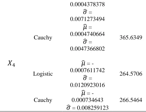
First step in identified distribution for each variable is with decide distribution candidate that will selected as an estimate from distribution variable. As for the distribution candidate election that will selected for each variable is using Cullen and Frey chart, that is the chart that show the closest theoretical distribution with distribution of variable based on skewness and kurtosis13. The next distribution election of the most suitable for each variable predictor performed with selecting distribution that have highest maximum likelihood function between selected distribution candidate. As for maximum likelihood values for each distribution candidate to each variable predictor that already identified with Cullen and Frey chart with estimate parameters is summarized on Table II.

TABLE II

MAXIMUM LIKELIHOOD

Variable Distributio n Estimate Parameter Log Likelihood Normal

̂ =

0.0003702703

̂ =

0.0092665104 362.1275 Cauchy

̂ =

0.0004498428

̂ =

0.0058591108 339.2576 Logistic

̂ =

0.0008406675

̂ =

0.0064906060 338.1017

Normal

̂ = 0.001107207

̂ = 0.011515479

338.0088

Cauchy

̂ =

0.0008503102

̂ =

0.0067734881 320.3173

Normal

̂ =

391.2614

0.0004378378

̂ =

0.0071273494 Cauchy

̂ =

0.0004740664

̂ =

0.0047366802 365.6349 Logistic

̂ =

-0.0007611742

̂ =

0.0120923016 264.5706 Cauchy

̂ =

-0.000734643

̂ = 0.008259123

266.5464

So the identified distribution with estimate parameter for each variable:

~ Bernoulli (0.46)

~ Normal (0.0003702703, 0.0092665104) ~ Logistic (0.0008406675, 0.0064906060) ~ Normal (0.0003702703, 0.0092665104) ~ Cauchy (-0.000734643, 0.008259123)

After distribution estimated for each variable is known, then Gaussian copula model will be built. This copula model will be used as the model for predict decrease or not the UNVR stock price on closing trading session at Indonesian Stock Exchange. The Copula marginal distribution composer is the distribution from variables that used as variable predictor ( , , , ). As for Gaussian copula model that formed at this research are as follows:

(

)

(

)

(

)

(

)

(

))

with

(

) is standard normal cumulative

distribution function that have mean 0 and standard deviation 1, and is cumulative distribution function from each variable predictor. While

is multivariate

normal cumulative distribution function with

and

.

is correlation matrix, that is:

[ ]

(4)

258 Copyright © 2016. Vandana Publications. All Rights Reserved.

(

)

( )

_{| |}

[( ) ₍

)]

Closing stock price prediction at this research is done with using data simulation that contains 500000 observations that built from Gaussian copula model. Because prediction process is done with big size data simulation, so illustration how algorithm run if using small size data will be given.

Data on Table III is simulation data that obtained from generate 10 observations. At the simulation data, each variable has been spread as the distribution has been suspected. Furthermore distance measurement between observations on training data with observation on simulation data which contained at Table III based on variables predictor will be calculated. As for this illustration, observation that used is first 5 observations on training data.

TABLE III SIMULATION DATA

Obs. Variable

1 0 0.0107730 0.0175383 0.0089007 0.0108510

2 1 0.0040080 0.0096347 0.0022212 -0.0033089

3 1 0.0037076

-0.0080205 0.0026203 0.0282461

4 1 -0.0224772

-0.0175178

-0.0173457 0.0045902

5 1 0.0053026 0.0096901 0.0044412 -0.1374158

6 1 0.0000235 0.0046331 0.0044760 -0.0011075

7 1 -0.0004300

-0.0038114

-0.0017429

-0.0057177

8 0 -0.0028557

-0.0114195

-0.0022133

-0.0151261

9 0

-0.0031188 0.0090715

-0.0012239 0.0022628

10 0 0.0087698

-0.0019969 0.0042450 0.0099822

For observation jth distance on training data with

ith on simulation data

(

), obtained using Euclidean

distance formula as for :

√( ) ( ) ( ) ( )

After distance calculation

(

) had been done

for all i and j, distance matrix sized

as seen at

Table IV obtained. At this distance matrix, the rows state observation amount from simulation data and the columns state observation amount from training data.

TABLE IV DISTANCE MATRIX

Row Column

1 2 3 4 5

1 0.060 0.014 0.083 0.061 0.041 2 0.042 0.011 0.069 0.064 0.023 3 0.058 0.031 0.104 0.032 0.056 4 0.035 0.048 0.091 0.049 0.046 5 0.118 0.140 0.067 0.192 0.114 6 0.040 0.012 0.072 0.060 0.025 7 0.029 0.020 0.071 0.060 0.023 8 0.018 0.030 0.066 0.068 0.022 9 0.043 0.017 0.075 0.057 0.027 10 0.046 0.012 0.085 0.050 0.039

After distance matrix obtained, the next step is make matrix prediction data with add new column into distance matrix that cells from the column are variable response values from simulation data. So matrix prediction data obtained as the Table 5.

TABLE V PREDICTION MATRIX

Row Column

1 2 3 4 5 6

1 0.060 0.014 0.083 0.061 0.041 0 2 0.042 0.011 0.069 0.064 0.023 1 3 0.058 0.031 0.104 0.032 0.056 1 4 0.035 0.048 0.091 0.049 0.046 1 5 0.118 0.140 0.067 0.192 0.114 1 6 0.040 0.012 0.072 0.060 0.025 1 7 0.029 0.020 0.071 0.060 0.023 1 8 0.018 0.030 0.066 0.068 0.022 0 9 0.043 0.017 0.075 0.057 0.027 0 10 0.046 0.012 0.085 0.050 0.039 0

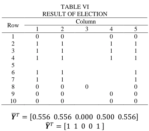
Furthermore prediction value for each observation from first 5 observations on training data obtained with selecting values from column 6 matrix prediction data first that match with values from each other columns, there is column 1 until 5, that have value not more than 0.067a). The result of this election can be seen at Table VI. After the values obtained, the next step is calculate average value from each column. The average result that will be obtain lie between 0 until 1. As for average calculated results lie on mean vector

(

̅). Then with rounding off

became 1 for average value more than 0.5 and rounding off became 0 for otherwise, so prediction result obtained for

a_{On the real prediction process at this research, bound value}

(5)

first 5 observation from training data as contained at

prediction vector (

̂)

.

TABLE VI RESULT OF ELECTION

Row Column

1 2 3 4 5

1 0 0 0 0

2 1 1 1 1

3 1 1 1 1

4 1 1 1 1

5

6 1 1 1

7 1 1 1

8 0 0 0 0

9 0 0 0 0

10 0 0 0 0

̅

_{[ ]}

̂

_{[ ]}

Evaluating prediction result aims to see prediction accuracy rate and prediction error rate that done with using simulation data that sized 500000 observations. Evaluation is done with Confusion Matrix that the values for each cell obtained from prediction result data. Based on prediction result data, obtained confusion matrix as follow:

Prediction Actual Sum of Prediction

̂ 47 22 69

̂ 13 29 42

Sum of

Actual 60 51 111

Furthermore evaluation is done with calculate accuracy rate and APER value (Apparent Error Rate) based on the result obtained on the confusion matrix. Accuracy value is obtained with calculate proportion observation amount value that predicted appropriately, toward the whole observation amount. While APER value obtained with calculate proportion observation amount value that prediction result not appropriate with actual value, toward the whole observation amount. As for calculation result this two evaluations are summarized at table VII.

TABLE VII

EVALUATING PREDICTION Evaluation Evaluation

Measurement

Proportion Percentage

Prediction

Accuracy Accuracy 0.6847 68.47% Prediction Error APER 0.3153 31.53%

Based on the table above, prediction result accuracy of closing stock price UNVR condition with the predictors are the opening index LQ-45 condition, the opening index Consumer Good condition, opening index Jakarta Composite Index condition, and opening stock price WIIM condition is 68.47% with error prediction rate is 31.53%.

V. CONCLUSION

Based on this research can conclude that Gaussian copula model can be used to do classification analysis, in this case is predicting closing stock price UNVR condition into one of two category, increase (0) or decrease (1). This classification or prediction is done with simulation data, with selecting observations on simulation data that have distance less than 0.004 with each observation at data. As for accuracy from the classification with Gaussian copula model is 68.47% with classification error rate 31.53%.

REFERENCES

[1] Moran PAP. Statistical Inference with Bivariate Gamma Distributions. Biometrika. 54: 385:394. 1969. [2]Gumbel EJ. Bivariate Exponential Distribution. Journal of The American Statistical Association. 55: 698-707. 1960.

[3] Salamah M, Kuswanto H. Identifikasi Struktur Dependensi dengan Copula (Aplikasi pada Data Klimatologi). Journal Cauchy. 1(2). ISSN 2086-0328. 2010.

[4] Sungur EA. Note on Directional Dependence in Regression Setting. Commun Stat: Theory Methods. 34 (9-10): 1957-1965. 2005.

[5] Scholzel C. Multivariate Non-Normally Distributed Random Variable in Climate Research-Introduction to Copula Approach. Germany: University of Born. 2008. [6] Ratih ID. Penaksiran Parameter pada Copula Regression (Studi Kasus: Pemodelan Luas Panen Padi di Kabupaten Jember, Jawa Timur). Surabaya: Institut Teknologi Sepuluh Nopember. 2014.

[7] Embrechts P, Lindskog F, McNeil A. Modelling Dependences with Copulas and Applications to Risk Management. Switzerland: Department of Mathematics. 2001.

[8] Aas K. Modelling The Dependence Structure of Financial Assets: A Survey of Four Copulas. Samba. 22(4):18. 2004.

[9] McNeil AJ, Frey R, Embrechts P. Quantitative Risk Management: Concepts and Techniques. Princeton: Princeton University Press. 2005.

(6)

[11] Voisin A, Krylov V, Moser G, Serpico SB, Zerubia J.

Classification of Very High Resolution SAR Images of Urban Areas Using Copulas and Texture in a Hierarchical Markov Random Field Model. IEEE Geoscience and Remote Sensing Letters. 10(1): 96-100. 2012.

[12] Nelsen RB. An Introduction to Copulas. Portland: Springer. 2005.