Efficient voice activity detection algorithm using long-term spectral flatness measure

(1)

R E S E A R C H

Open Access

Efficient voice activity detection algorithm

using long-term spectral flatness measure

Yanna Ma

*

and Akinori Nishihara

Abstract

This paper proposes a novel and robust voice activity detection (VAD) algorithm utilizing long-term spectral flatness measure (LSFM) which is capable of working at 10 dB and lower signal-to-noise ratios(SNRs). This new LSFM-based VAD improves speech detection robustness in various noisy environments by employing a low-variance spectrum estimate and an adaptive threshold. The discriminative power of the new LSFM feature is shown by conducting an analysis of the speech/non-speech LSFM distributions. The proposed algorithm was evaluated under 12 types of noises (11 from NOISEX-92 and speech-shaped noise) and five types of SNR in core TIMIT test corpus. Comparisons with three modern standardized algorithms (ETSI adaptive multi-rate (AMR) options AMR1 and AMR2 and ITU-T G.729) demonstrate that our proposed LSFM-based VAD scheme achieved the best average accuracy rate. A long-term signal variability (LTSV)-based VAD scheme is also compared with our proposed method. The results show that our

proposed algorithm outperforms the LTSV-based VAD scheme for most of the noises considered including difficult noises like machine gun noise and speech babble noise.

1 Introduction

Voice activity detection (VAD) is a method to discriminate speech segments from input noisy speech. It is an integral part to many speech and audio processing applications and is widely used within the field of speech communica-tion for achieving high coding efficiency and low bit rate transmission. Examples include noise reduction for digi-tal hearing aid devices [1], mobile communication services [2], voice recognition systems [3], compression [4], and speech coding [5].

A typical VAD system consists of two core parts: feature extraction and speech/non-speech decision mechanism. Researchers have proposed a variety of features exploit-ing different properties of speech and noise to achieve better VAD performance. In early VAD algorithms, short-term energy [6] and zero-crossing rate [7] were widely used features because of their simplicity. However, the performance degrades easily when faced with low signal-to-noise ratio (SNR) or non-stationary background noise. To solve this problem, robust acoustic features such as spectrum [8], autocorrelation [9], power in the band-limited region [10], and higher-order statistics [11] have

*Correspondence: [email protected]

Department of Communications and Integrated Systems, Tokyo Institute of Technology, Tokyo 152-8552, Japan

been proposed for VAD. Most of those methods assume the background noise to be stationary during a certain period; thus, they are sensitive to changes in SNR of the observed signal. Some works [12,13] proposed noise esti-mation and adaptation for improving VAD robustness, but those methods are computationally expensive. Most of those features mentioned work sufficiently well in station-ary noise and higher than 10-dB SNR cases. When facing with lower SNR cases or when the background noise con-tains complex audible events appearing occasionally, such as babble noise in a cafeteria and machinery noise in a factory, there will be cases when most of the speech spec-trum is corrupted, which destroys the overall statistical as well as structural properties of the speech signal [14]. In general, VAD algorithms based on a particular feature or specific set of features are still far from efficient especially when they are operating in adverse acoustic conditions. Therefore, the VAD algorithm in low SNRs and some spe-cific noises such as speech babble noise and machine gun noise still remains challenging and requires the design of further robust features and algorithms.

All VAD features mentioned are extracted from the short-term analysis frames (usually 20 to 40 ms), and decisions are made at each frame. In contrast with the use of frame level features, Ramirez et al. [12] proposed

(2)

the use of a long-term spectral divergence feature to dis-criminate speech from noise. It requires average noise spectrum magnitude information which is not accurately available in practice. Moreover, Ghosh et al. [15] proposed a long-term signal variability (LTSV)-based VAD which uses a very long window to estimate the averaged spec-trogram as well as for computing long-term entropies of each frequency band. This LTSV-based VAD yields a great improvement for SNRs smaller than 5 dB but becomes saturated when SNRs are higher than 5 dB.

Spectral flatness is a measure of the width, uniformity, and noisiness of the power spectrum. A high spectral flat-ness indicates that the spectrum has a similar amount of power in all spectral bands, and the graph of the spectrum would appear relatively flat and smooth; this would sound similar to white noise. A low spectral flat-ness indicates that the spectral power is less uniform in frequency structure, and this would typically sound like speech. Therefore, the analysis over a long window for exploiting the spectral flatness of the signal will be beneficial for distinguishing speech from noise. In this paper, we propose a novel VAD algorithm based on

long-term spectral flatness measure (LSFM). The discrimina-tive power of the proposed LSFM feature will be veri-fied by researching the distribution of LSFM measure for speech and non-speech in terms of their misclassification rate for various noises. We have experimentally evaluated its performance under a variety of noise types and SNR conditions.

The structure of the rest of this article is arranged as follows. Section 2 discusses the LSFM feature and its discriminative ability. Section 3 presents the proposed LSFM-based VAD algorithm including the choice for proper parameters and the design of an adaptive thresh-old. Section 4 contains the speech and noise database and metrics used in the evaluation. Section 5 provides the experimental results. Finally, a conclusion of this work and the discussion are given in Section 6.

2 Long-term spectral flatness measure and its discriminative power

Speech is a highly non-stationary signal, while back-ground noise can be considered to be stationary over relatively long periods. The rationale behind the LSFM

−10 −0.5 0 0.5 1 1.5

0.05 0.1 0.15 0.2 0.25 0.3 0.35 0.4

log 10(|LSFM|)

Normalized Count

White, SNR=−10dB, 25bins,R=2

Speech Non−speech

0 0.5 1 1.5 2 2.5

0 0.05 0.1 0.15 0.2 0.25 0.3 0.35 0.4

log 10(|LSFM|)

R=5

0 0.5 1 1.5 2 2.5

0 0.05 0.1 0.15 0.2 0.25 0.3 0.35 0.4

log 10(|LSFM|)

R=10

0 0.5 1 1.5 2 2.5

0 0.05 0.1 0.15 0.2 0.25 0.3 0.35 0.4

log₁₀(|LSFM|)

R=20

0 0.5 1 1.5 2 2.5

0 0.05 0.1 0.15 0.2 0.25 0.3 0.35 0.4

log₁₀(|LSFM|)

R=30

0 0.5 1 1.5 2 2.5

0 0.05 0.1 0.15 0.2 0.25 0.3 0.35 0.4

log₁₀(|LSFM|)

R=40

Error=21.98% Correct=78.02% SE=10.31% NE=11.67%

Error=17.78% Correct=82.22% SE=6.20% NE=11.58% Error=39.42%

Correct=60.58% SE=12.81% NE=26.61%

Correct=54.39% SE=15.10% NE=30.51%

(3)

feature is that the observed signal spectrum evinces more structure when the signal of interests is present compared to when it is absent. This increase in the structure of the signal may be characterized by a reduction in the flatness of the magnitude spec-trum of the short-time Fourier representation of the signal [16].

2.1 Long-term spectral flatness measure

The LSFM feature is computed using the spectra of the last R frames of the input signal x(n). The LSFM fea-ture,Lx(m), at the mth frame and across all the chosen frequency is then calculated by dividing the geometric mean of the power spectrum by the arithmetic mean of the power spectrum. To expand the dynamic range, it is measured on a logarithmic scale, ranging from zero to minus infinity as:

Lx(m)=

k

log₁₀GM(m,ωk)

AM(m,ω_k), (1)

where the geometric mean GM(m,ωk) and arithmetic mean AM(m,ωk)of the power spectrum is calculated as:

GM(m,ωk)= R

m

n=m−R+1

S(n,ωk), (2)

AM(m,ωk)= _R1 m

n=m−R+1

S(n,ωk). (3)

The short-time spectrumS(n,ωk)used in this research is estimated using the Welch-Bartlett method which aver-ages the spectral estimates ofMconsecutive frames. The expressions are

S(n,ωk)= _M1 n

p=n−M+1

|X(p,ωk)|2, (4)

X(p,ωk)=

Nw+(p−1)Nsh

l=(p−1)Nsh+1

w(l−(p−1)Nsh−1)x(l)e−jωkl,

(5)

−1 0 1 2

0 0.05 0.1 0.15 0.2 0.25 0.3 0.35 0.4 0.45

log

10(|LSFM|)

White, SNR=−5dB, 25bins,R=2

0 1 2 3

0 0.05 0.1 0.15 0.2 0.25 0.3 0.35 0.4 0.45

log

10(|LSFM|)

R=5

0 1 2 3

0 0.05 0.1 0.15 0.2 0.25 0.3 0.35 0.4 0.45

log

10(|LSFM|)

R=10

0 1 2 3

0 0.05 0.1 0.15 0.2 0.25 0.3 0.35 0.4 0.45

log

10(|LSFM|)

R=20

0 1 2 3

0 0.05 0.1 0.15 0.2 0.25 0.3 0.35 0.4 0.45

log

10(|LSFM|)

R=30

0 1 2 3

0 0.05 0.1 0.15 0.2 0.25 0.3 0.35 0.4 0.45

log

10(|LSFM|)

R=40 Error=32.36 %

Correct=67.64% SE=11.18% NE=21.18% Error=41.86%

Correct=58.14% SE=13.86% NE=28.00%

Error=21.65 % Correct=78.35% SE=8.86% NE=12.79%

Error=9.99 % Correct=90.01% SE=4.62% NE=5.37% Error=10.68%

Correct=89.32% SE=5.60% NE=5.08% Error=13.13%

Correct=86.87% SE=7.49% NE=5.64%

(4)

whereX(p,ωk)is the short-time Fourier transform coef-ficient at frequency ωk of the pth frame. w(i) is the short-time Hann window, where i ∈[ 0,Nw). Nw is the frame length andNshis the frame shift duration in terms

of samples.

According to AM-GM inequality, the geometric mean, GM(m,ω_k), is smaller than or equal to the arith-metic mean, AM(m,ω_k), with equality being achieved if and only if all S(n,ωk) are the same. Therefore, from Equation 1, we can conclude that the LSFM feature,Lx(m), is in the range(−∞, 0] with the maximum value acquired when the geometric mean is equal to the arithmetic mean.

2.2 The LSFM feature distributions of speech and non-speech

In this subsection, the distributions of the LSFM feature are investigated in order to clarify the motivation for uti-lizing the proposed LSFM feature as a VAD algorithm and demonstrate the discriminative power of this feature.

The test set consisting of 16 individual speakers (8 male, 8 female), each speaking 10 phonetically balanced English

sentences, is randomly chosen from the TIMIT training corpus [17]. The LSFM feature values were computed at every frame from noisy speech. The LSFM measure,

Lx(m), is considered to be LS+N(m) if there are speech samples between(m−R+1)th andmth frame. Other-wise, it is decided to be LN(m). The overlap area of the two distributions (LS+N andLN) is considered to be the error caused by misclassification. The lower the misclas-sification rate is, the better the separation. The sampling frequency of the test signal is 16 kHz, and the Hann win-dow has a length of 20 ms and a 10-ms shift.Mis fixed to be 10, and{ωk}is uniformly distributed between the fre-quency range 500 Hz to 4 kHz. The total misclassification error among these realizations ofLS+N andLN was com-puted by comparing with the phonetic level transcription [17] of the TIMIT training corpus.

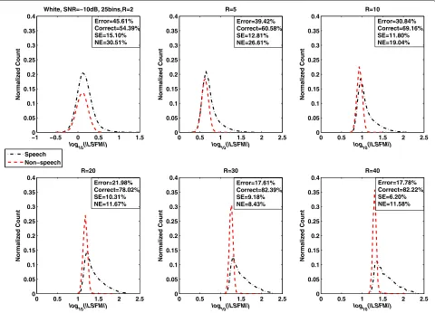
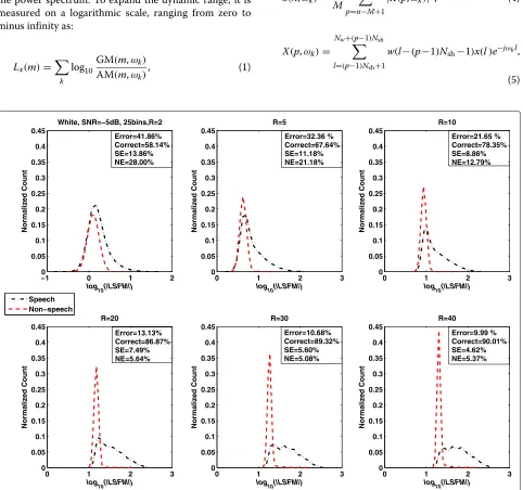
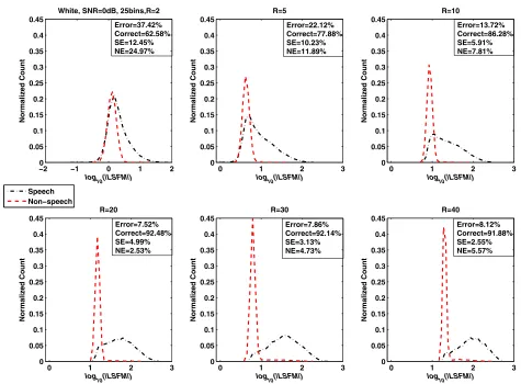
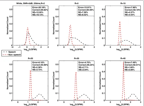
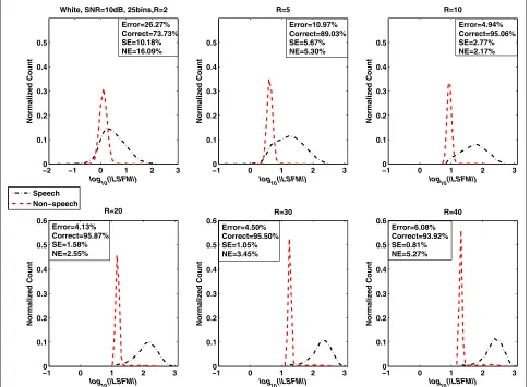
First, the distributions of the LSFM feature as a func-tion of the long-term window length (R = 2, 5, 10, 20, 30, and 40) for white noise at five SNR levels (−10, −5, 0, 5, and 10 dB) were studied. The results are shown in Figures 1, 2, 3, 4, and 5. The total misclassification

−20 −1 0 1 2

0.05 0.1 0.15 0.2 0.25 0.3 0.35 0.4 0.45

log

10(|LSFM|)

White, SNR=0dB, 25bins,R=2

0 1 2 3

0 0.05 0.1 0.15 0.2 0.25 0.3 0.35 0.4 0.45

log

10(|LSFM|)

R=5

0 1 2 3

0 0.05 0.1 0.15 0.2 0.25 0.3 0.35 0.4 0.45

log

10(|LSFM|)

R=10

0 1 2 3

0 0.05 0.1 0.15 0.2 0.25 0.3 0.35 0.4 0.45

log

10(|LSFM|)

R=20

0 1 2 3

0 0.05 0.1 0.15 0.2 0.25 0.3 0.35 0.4 0.45

log

10(|LSFM|)

R=30

0 1 2 3

0 0.05 0.1 0.15 0.2 0.25 0.3 0.35 0.4 0.45

log

10(|LSFM|)

R=40 Error=22.12%

Correct=77.88% SE=10.23% NE=11.89%

Correct=62.58% SE=12.45% NE=24.97%

(5)

−20 −1 0 1 2 3 0.1

0.2 0.3 0.4 0.5

log₁₀(|LSFM|)

0 1 2 3

0 0.1 0.2 0.3 0.4 0.5

log₁₀(|LSFM|)

R=5

0 1 2 3

0 0.1 0.2 0.3 0.4 0.5

log₁₀(|LSFM|)

R=10

0 1 2 3

0 0.1 0.2 0.3 0.4 0.5

log₁₀(|LSFM|)

R=20

0 1 2 3

0 0.1 0.2 0.3 0.4 0.5

log₁₀(|LSFM|)

R=30

0 1 2 3

0 0.1 0.2 0.3 0.4 0.5

log₁₀(|LSFM|)

R=40

Error=7.49% Correct=92.51% SE=1.60% NE=5.89% Error=7.90% Correct=92.10% SE=4.37% NE=3.53% Error=15.91%

Correct=84.09% SE=7.39% NE=8.52%

Correct=93.90% SE=2.38% NE=3.72% Error=30.18% Correct=69.82% SE=12.05% NE=18.13%

Figure 4LSFM measure as a function of long-term window length (R) in additive white noise (SNR = 5 dB).

error (Error), accuracy rate (Correct), speech detection error (SE), and non-speech detection error (NE) are dis-played on the upper or lower right of each subfigure. The total misclassification error was reduced by 61.4% (−10 dB), 74.5% (−5 dB), 79.0% (0 dB), 84.3% (5 dB), and 82.9% (10 dB) when the window lengthRwas increased from 2 to 30 frames. The percentage is the ratio between the reduced misclassification error (whenRwas changed from 2 to 30 frames) and the misclassification error when

Rwas 2.

The distributions of the LSFM feature for all 12 kinds of noises at 0-dB SNR were investigated.Mis fixed to be 10, andRis chosen to be 30. The discriminative power of this LSFM feature can be measured by the separateness of its distribution for speech and non-speech. As shown in Figures 6, 7, and 8, there is overlap between the his-tograms of log₁₀(LS+N)and log₁₀(LN). We calculated the total misclassification error which is the sum of the speech detection error and non-speech detection error. From the figures, we can conclude that for most noises considered

(9 out of 12 kinds of noises), the proposed LSFM fea-ture resulted in a misclassification error smaller than 10%: white (7.86%), pink (7.75%), tank (7.47%), military vehi-cle (7.75%), jet cockpit (9.32%), HF channel (8.30%), F-16 cockpit (8.89%), car interior (8.14%), and speech shaped (7.84%). For factory floor (25.86%), machine gun (45.42%), and speech babble (24.08%), the misclassification errors were comparatively high. The factory floor is that of cutting noise, that of the machine gun is impulsive in nature, and that of speech babble is speechlike. One pos-sible reason for the poor performance is the mismatch of

MandR.

(6)

−20 −1 0 1 2 3 0.1

0.2 0.3 0.4 0.5

log₁₀(|LSFM|)

−1 0 1 2 3

0 0.1 0.2 0.3 0.4 0.5

log₁₀(|LSFM|)

R=5

−10 0 1 2 3

0.1 0.2 0.3 0.4 0.5

log₁₀(|LSFM|)

R=10

−10 0 1 2 3

0.1 0.2 0.3 0.4 0.5 0.6

log₁₀(|LSFM|)

R=20

−1 0 1 2 3

0 0.1 0.2 0.3 0.4 0.5 0.6

log₁₀(|LSFM|)

R=30

−10 0 1 2 3

0.1 0.2 0.3 0.4 0.5 0.6

log₁₀(|LSFM|)

R=40 Error=26.27%

Correct=73.73% SE=10.18% NE=16.09%

Figure 5LSFM measure as a function of long-term window length (_R) in additive white noise (SNR = 10 dB).

commonly employed for spectrum estimation, but it is well known that the periodogram is an inconsistent spectral estimator. According to [8], the Welch-Bartlett method [19] was found to give a good trade-off between variance reduction and spectral resolution reduction. Therefore, in our proposed algorithm, the signal spectrum is estimated using the Welch-Bartlett method.

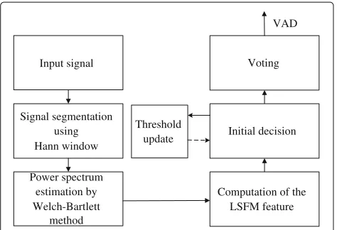
A block diagram of the proposed LSFM-based VAD algorithm is shown in Figure 9. The algorithm can be described as follows. The input speech signal is decom-posed into frames of 20 ms in length with an overlap of 10 ms by the Hann window. The spectrum of the segmented signal is estimated using the Welch-Bartlett method. At the mth frame, the LSFM feature Lx(m) is computed using the previousRframes. The initial deci-sion about whether there contains speech in the last R frames is made through the comparison with an adap-tive threshold. The initial decision is denoted by VINL.

If there is a speech frame existing over the previous R frames ending at themth frame,VINL(m)=1; otherwise,

VINL(m) = 0 and there are only non-speech frames over

the previousRframes. We adopt the voting scheme pro-posed by Ghosh et al. [15] to make the final VAD decisions on a 10-ms interval. First, the initial decisions,VINL(m),

VINL(m+1),. . .,VINL(m+R−1), are collected for those

long windows which overlap with the target 10-ms inter-val. Then, the target 10-ms interval is marked to be speech if there is 80% or above of those initial decisions that contain speech; otherwise, it is marked as non-speech. The 80% was gotten empirically, which provided the max-imum VAD accuracy for most noises tested over five SNR levels.

In general, speech is a low-pass signal, and the fre-quency range of 500 Hz to 4 kHz is crucial for speech intelligibility [20]. Hence, for a better discrimination, the start bin,ks, and the end frequency bin,ke, are calculated by:

ks=NDFT(

500

(7)

0 0.5 1 1.5 2 2.5 3 3.5 4 0

0.1 0.2 0.3 0.4 0.5

log₁₀(|LSFM|)

White noise, SNR=0dB, 25bins

0 0.5 1 1.5 2 2.5 3 3.5 4

0 0.1 0.2 0.3 0.4 0.5

log₁₀(|LSFM|)

Pink noise, SNR=0dB, 25bins

0 0.5 1 1.5 2 2.5 3 3.5 4

0 0.1 0.2 0.3 0.4 0.5

log₁₀(|LSFM|)

Tank noise, SNR=0dB, 25bins

0 0.5 1 1.5 2 2.5 3 3.5 4

0 0.1 0.2 0.3 0.4 0.5

log₁₀(|LSFM|)

Military vehicle noise, SNR=0dB, 25bins

Correct=92.14% SE=3.13% NE=4.73%

Figure 6Histogram of the logarithmic LSFM measure for white, pink, tank, and military vehicle noises (SNR = 0 dB).Upper left: white noise, upper right: pink noise, lower left: tank noise, and lower right: military vehicle noise.

ke=NDFT(

4, 000

fs ), (7)

in whichfsis the sampling frequency andNDFTis the order

of Discrete Fourier Transform (DFT) which is used to cal-culate the spectral estimate of the observed signal. In our experiment,f_s = 16 kHz andNDFT = 512. The

frequen-cies,ω_k , are uniformly distributed between 500 Hz and 4 kHz.

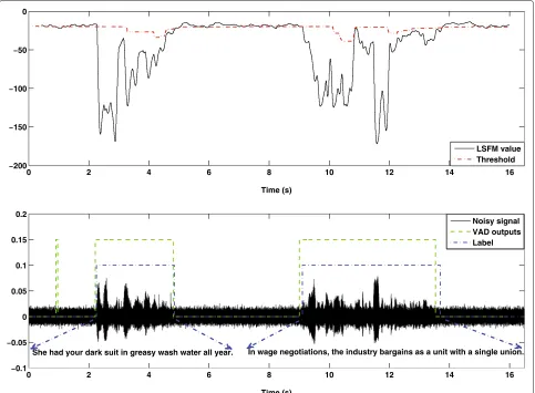
An illustrative example of the VAD output is shown in Figure 10. A high spectral flatness indicates that the spec-trum has a similar amount of power in all spectral bands, which would sound similar to white noise, and the graph of the spectrum would appear relatively flat and smooth. A low spectral flatness indicates that the spectral power is concentrated in a relatively small number of bands; this means that the spectrum is more organized, and the graph of the spectrum would appear ‘spiky’. Hence, the spectral flatness measure is a good feature for VAD.

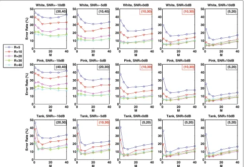
3.1 Selection ofMandR

MandR are parameters used for computing the LSFM featureLx. We want to choose the appropriateMandR so that the separateness of the distribution for noise and speech is maximized since the more it is separated, the better the final VAD decision is. The total misclassifica-tion errors (sum of speech detecmisclassifica-tion error and non-speech detection error) for all combinations ofM(1, 5, 10, 20, 30, and 40) andR(5, 10, 20, 30, and 40) are computed over 12 types of noise for five SNR levels (−10,−5, 0, 5, and 10 dB). The test speech set is the same with the one we used for the demonstration of the discriminative power of the proposed LSFM feature in Section 2.2.

The total misclassification error as a function of

different combinations of M and R is shown in

(8)

0 0.5 1 1.5 2 2.5 3 3.5 4 0

0.1 0.2 0.3 0.4 0.5

log₁₀(|LSFM|)

Jet cockpit noise, SNR=0dB, 25bins

Speech Non speech

0 0.5 1 1.5 2 2.5 3 3.5 4

0 0.1 0.2 0.3 0.4 0.5

log₁₀(|LSFM|)

HF channel noise, SNR=0dB, 25bins

0 0.5 1 1.5 2 2.5 3 3.5 4

0 0.1 0.2 0.3 0.4 0.5

log₁₀(|LSFM|)

F 16 cockpit noise, SNR=0dB, 25bins

0 0.5 1 1.5 2 2.5 3 3.5 4

0 0.1 0.2 0.3 0.4 0.5

log₁₀(|LSFM|)

Factory floor noise, SNR=0dB, 25bins Error=9.32%

Correct=90.68% SE=2.77% NE=6.55%

Correct=91.11% SE=2.39% NE=6.50%

Figure 7Histogram of the logarithmic LSFM measure for jet cockpit, HF channel, F-16 cockpit, and factory floor noises (SNR = 0 dB).

Upper left: jet cockpit noise, upper right: HF channel noise, lower left: F-16 cockpit noise, and lower right: factory floor noise.

which appeared most frequently ( M = 10 appeared 25 times out of the 60 subfigures in total;R = 30 also appeared 25 times out of 60 subfigures in total). This fixed combination (10, 30) is then adopted for all the following tests.

Furthermore, from Figures 11, 12, 13, and 14, we observe that for the sameRvalue, ifMis increased from 1 to 10, the total misclassification error is decreased for most cases tested. However, when M is larger than 10, even if M is increased, the total misclassification error stops decreasing any further. This observation verified the choice of 10 to be the optimal value ofM.

It is also worth mentioning that for those noise types and SNR levels whose optimal MandR combination is not (10, 30), the fixed combination (10, 30) still works well. Table 1 shows the points that the total misclassification error of adopting the fixed combination (10, 30) is worse (higher error value) than utilizing the best combination ofMandRfor each noise type and SNR level shown in

the subfigures. Except for cutting factory floor noise and impulsive machine gun noise, the differences are all less than five points.

(9)

0 0.5 1 1.5 2 2.5 3 3.5 4 0

0.1 0.2 0.3 0.4 0.5

log₁₀(|LSFM|)

Car interior noise, SNR=0dB, 25bins

Speech Non speech

0 0.5 1 1.5 2 2.5 3 3.5 4

0 0.1 0.2 0.3 0.4 0.5

log₁₀(|LSFM|)

Machine gun noise, SNR=0dB, 25bins

0 0.5 1 1.5 2 2.5 3 3.5 4

0 0.1 0.2 0.3 0.4 0.5

log₁₀(|LSFM|)

Speech babble noise, SNR=0dB, 25bins

0 0.5 1 1.5 2 2.5 3 3.5 4

0 0.1 0.2 0.3 0.4 0.5

log₁₀(|LSFM|)

Speech shaped noise, SNR=0dB, 25bins

Figure 8Histogram of the logarithmic LSFM measure for car interior, machine gun, speech babble, and speech-shaped noises (SNR =

0 dB).Upper left: car interior noise, upper right: machine gun noise, lower left: speech babble noise, and lower right: speech-shaped noise.

Input signal

Signal segmentation using Hann window

Power spectrum estimation by Welch-Bartlett

method

Computation of the LSFM feature Initial decision

Voting

Threshold update

VAD

Figure 9Block diagram of the proposed LSFM-based VAD algorithm.

more misclassification errors compared to the case when

Mis 1.

3.2 Adaptive threshold

UnlikeMandR, a fixed threshold would lose its efficiency when facing varying acoustic environments. Therefore, it is more suitable to design an adaptive threshold [22]. From Equations 2 to 4, we can conclude that(R+M−1)frame (0.39 s for fixed R = 30 and M = 10) information is needed to acquire the first LSFM feature value. In our implementations, the initial 1.39 s of the test signalx(n)is always assumed to be non-speech. From this 1.39 s ofx(n), 100 realizations ofLNcan be collected and saved toψINL.

The threshold is initialized to be

THRINL=min(ψINL). (8)

(10)

0 2 4 6 8 10 12 14 16 200

150 100 50 0

Time (s)

LSFM value Threshold

0 2 4 6 8 10 12 14 16

0.1 0.05 0 0.05 0.1 0.15 0.2

Time (s)

Noisy signal VAD outputs Label

In wage negotiations, the industry bargains as a unit with a single union. She had your dark suit in greasy wash water all year.

Figure 10Illustrative example of the adaptive threshold and the VAD output, white noise, SNR = 0 dB.The upper figure shows the LSFM value and the corresponding adaptive threshold for each frame. The lower figure shows the VAD output decisions and the ground truth, namely ‘Label’. The two sentences are as follows: (1) She had your dark suit in greasy wash water all year; (2) in wage negotiations, the industry bargains as a unit with a single union.

the LSFM measures of the last 100 long window ending at the mth frame which was decided as including non-speech information only. The adaptive threshold for the

mth frame is then updated as:

THR(m)=λ×min(ψS+N)+(1−λ)×max(ψN), (9)

whereλis the parameter of the convex combination. We experimentally found that λ = 0.55 results in the max-imum accuracy rate in VAD decisions over the TIMIT training set.

4 Evaluation setup

The proposed VAD algorithm was trained and tested using a speech database that is phonetically balanced. The system was evaluated using the error rate and accuracy rate metrics.

4.1 Database description

(11)

0 20 40 0 10 20 30 40 50 M

Error Rate (%)

White, SNR= 10dB

0 20 40

0 10 20 30 40 50 M White, SNR= 5dB

0 20 40

0 10 20 30 40 50 M White, SNR=0dB

0 20 40

0 10 20 30 40 50 M White, SNR=5dB

0 20 40

0 10 20 30 40 50 M White, SNR=10dB R=5 R=10 R=20 R=30 R=40

0 20 40

0 10 20 30 40 50 M

Error Rate (%)

Pink, SNR= 10dB

0 20 40

0 10 20 30 40 50 M Pink, SNR= 5dB

0 20 40

0 10 20 30 40 50 M Pink, SNR=0dB

0 20 40

0 10 20 30 40 50 M Pink, SNR=5dB

0 20 40

0 10 20 30 40 50 M Pink, SNR=10dB

0 20 40

0 10 20 30 40 50 M

Error Rate (%)

Tank, SNR= 10dB

0 20 40

0 10 20 30 40 50 M Tank, SNR= 5dB

0 20 40

0 10 20 30 40 50 M Tank, SNR=0dB

0 20 40

0 10 20 30 40 50 M Tank, SNR=5dB

0 20 40

0 10 20 30 40 50 M Tank, SNR=10dB

(30,40) (10,40) (5,20)

(5,20) (20,30)

(40,40)

(20,30) (5,20) (5,20) (5,20)

(10,30) (10,30)

(10,30)

Figure 11Total misclassification error as a function of_Mand_Rcombination for white, pink, and tank noises.Upper row: white noise, middle row: pink noise, and lower row: tank noise. SNR=−10,−5, 0, 5, and 10 dB.

The noise of 11 categories taken from the NOISEX-92 database [21] and speech-shaped noise are added at five different SNR levels (−10,−5, 0, 5, and 10 dB) to the sig-nal concatenated by all 240 sentences. The noise samples from the NOISEX-92 database are resampled to 16 kHZ according to the experiment requirement. Among the 12 kinds of noises, white noise and pink noise are stationary noises while others are all non-stationary noises, namely tank, military vehicle, jet cockpit, HF channel, F-16 cock-pit, factory floor, car interior, machine gun, speech babble, and speech-shaped noises. The test set for each noise and SNR thus consisted of 28.10 min of noisy speech of which 62.51% was only noise.

4.2 Performance evaluation

Performance of a VAD algorithm can be evaluated both subjectively and objectively. In general, subjective evalu-ation is done through a listening test, and VAD decision errors are detected based on human perception [24]. On the other hand, objective evaluation relies on a mathemat-ical criterion for judging. However, subjective listening

tests like ABC [24] fail to consider the effect of the false alarm which is inappropriate for a thorough evaluation of a VAD algorithm [8]. Therefore, the objective evaluation scheme proposed by Freeman et al. [2] was adopted to evaluate the performance of the proposed VAD algorithm.

4.2.1 Error rate

The four traditional parameters that describe the error rate are as follows:

• Front-end clipping (FEC). Clipping introduced in passing from noise to speech activity.

• Mid-speech clipping (MSC). Clipping due to speech misclassified as noise in an utterance.

• Noise detected as speech (NDS). Noise detected as speech within a silence period.

• Carry over (OVER). Noise interpreted as speech due to the VAD flag remaining active in passing from speech activity to noise.

(12)

0 20 40 0 10 20 30 40 50 M

Error Rate (%)

Military vehicle, SNR=−10dB

0 20 40

0 10 20 30 40 50 M

Military vehicle, SNR=−5dB

0 20 40

0 10 20 30 40 50 M

Military vehicle, SNR=0dB

0 20 40

0 10 20 30 40 50 M

0 20 40

0 10 20 30 40 50 M

R=5 R=10 R=20 R=30 R=40

0 20 40

0 10 20 30 40 50 M

Error Rate (%)

Jet cockpit, SNR=−10dB

0 20 40

0 10 20 30 40 50 M Jet cockpit, SNR=−5dB

0 20 40

0 10 20 30 40 50 M Jet cockpit, SNR=0dB

0 20 40

0 10 20 30 40 50 M

Error Rate (%)

HF channel, SNR=−10dB

0 20 40

0 10 20 30 40 50 M HF channel, SNR=−5dB

0 20 40

0 10 20 30 40 50 M HF channel, SNR=0dB

0 20 40

(5,20) (5,20) (5,10) (5,10) (5,10)

(10,20)

(5,20) (10,30)

(30,40)

(10,30) (10,30) (10,30)

(10,30)

(10,20) (10,20)

Figure 12Total misclassification error as a function ofMandRcombination for military, jet cockpit, and HF channel noises.Upper row: military noise, middle row: jet cockpit noise, and lower row: HF channel noise. SNR=−10,−5, 0, 5, and 10 dB.

rejection, while NDS and OVER are indicators of false acceptance. Thus, in order to obtain the best over-all system performance, over-all four parameters should be minimized.

4.2.2 Accuracy rate

Although the method described above provides useful objective information concerning the performance of a VAD algorithm, it only gives the error rate of the system. Parameters which describe the accuracy rate are needed for a thorough analysis of the detection results. Three parameters concerning the accuracy rate are described as follows:

• CORRECT . They are correct decisions made by VAD algorithm.

• Speech hit rate (HR1). Speech frames that are correctly detected among all speech frames.

• Non-speech hit rate (HR0). Non-speech frames that are correctly detected among all non-speech frames.

Among the three parameters, HR1 and HR0 define the fraction of all actual speech frames or non-speech frames that are correctly detected as speech frames or

non-speech frames, respectively [12]. The speech hit rate and non-speech hit rate are calculated as follows:

HR1= N1,1

Nref 1

HR0= N0,0

Nref 0

, (10)

whereN₁refandN₀refare the numbers of real speech and non-speech frames in the whole database, respectively, whileN1,1andN0,0 are the numbers of speech and

non-speech frames correctly classified. The overall accuracy rate (CORRECT) is then defined as:

CORRECT= N1,1+N0,0

Nref 1 +N0ref

. (11)

All three parameters should be maximized to get the best performance.

5 Simulation results

(13)

0 20 40 0 10 20 30 40 50 M

Error Rate (%)

F 16 cockpit, SNR= 10dB

0 20 40

0 10 20 30 40 50 M

F 16 cockpit, SNR= 5dB

0 20 40

0 10 20 30 40 50 M

F 16 cockpit, SNR=0dB

0 20 40

0 10 20 30 40 50 M

0 20 40

0 10 20 30 40 50 M

R=5 R=10 R=20 R=30 R=40

0 20 40

0 10 20 30 40 50 M

Error Rate (%)

Factory floor, SNR= 10dB

0 20 40

0 10 20 30 40 50 M

Factory floor, SNR= 5dB

0 20 40

0 10 20 30 40 50 M

Factory floor, SNR=0dB

0 20 40

0 10 20 30 40 50 M

0 20 40

0 10 20 30 40 50 M

0 20 40

0 10 20 30 40 50 M

Error Rate (%)

Car interior, SNR= 10dB

0 20 40

0 10 20 30 40 50 M

Car interior, SNR= 5dB

0 20 40

0 10 20 30 40 50 M Car interior, SNR=0dB

0 20 40

0 10 20 30 40 50 M Car interior, SNR=5dB

0 20 40

0 10 20 30 40 50 M

Car interior, SNR=10dB

(5,10)

(10,30) (5,20)

(10,30)

(1,30)

(1,30) (1,40) (1,30) (1,30)

(5,10) (5,10) (5,10) (5,10) (5,20) (5,30)

Figure 13Total misclassification error as a function of_Mand_Rcombination for F-16 cockpit, factory floor, and car interior noises.Upper row: F-16 cockpit noise, middle row: factory floor noise, and lower row: car interior noise. SNR=₋10,₋5, 0, 5, and 10 dB.

three schemes were taken from the authors’ C implemen-tations [27,28], respectively.

One important aspect of the comparison is the different frame lengths used. The proposed schemes, the G.729B VAD and LTSV-based VAD, produce a decision every 10 ms, while the AMR VADs need 20 ms. In order to be comparable, the frame-wise VAD decisions produced by the AMR VADs were compared to a set of reference labels generated every 20 ms from the TIMIT phonetic level transcription. Meanwhile, the proposed schemes, the G.729B VAD and LTSV-based VAD, were compared to a set of reference labels generated every 10 ms from the TIMIT phonetic level transcription. The TIMIT utter-ances were down-sampled to 8 kHz for the software implementations of the G.729B VAD and AMR VADs. The final VAD decisions were made, and the accuracy rate and error rate were computed for 12 noises and five SNRs.

5.1 Performance average over all twelve kinds of noises In Figure 16, the proposed LSFM-based VAD is com-pared with three standards and LTSV-based VAD in terms of accuracy rate and error rate for SNR levels ranging from −10 to 10 dB. Note that the results in Figure 16

are averaged values for all 12 noises. The first row of the figure shows the accuracy rates which include COR-RECT, HR1, and HR0. The behavior of the different VADs is analyzed. G.729B suffers poor CORRECT(62.74% at −10 dB) and HR1 (33.62% at−10 dB) with the increas-ing noise level, while it keeps a steady and relatively high HR0 for the whole range of SNRs (80.33% on average). AMR1 performs much better than G.729B for both COR-RECT and HR1 while suffering degradation of HR0 when the SNR level is increased. AMR2 improves considerably over AMR1 in CORRECT mainly because of the high HR0 over all SNRs (88.96% on average) while yielding similar HR1 with AMR1. LTSV performs very well under low SNR conditions (80.73% CORRECT at−10 dB) but becomes saturated (around 91% since 5 dB) at higher SNRs. Our proposed LSFM-based VAD yields the best CORRECT for all SNRs and shows a steady improvement with the increased SNR.

(14)

0 20 40 0

20 40 60

M

Error Rate (%)

Machine gun, SNR= 10dB

0 20 40

0 20 40 60

M

Machine gun, SNR= 5dB

0 20 40

0 20 40 60

M

Machine gun, SNR=0dB

0 20 40

0 20 40 60

M

0 20 40

0 20 40 60

M

R=5 R=10 R=20 R=30 R=40

0 20 40

0 20 40 60

M

Error Rate (%)

Speech babble, SNR= 10dB

0 20 40

0 20 40 60

M

Speech babble, SNR= 5dB

0 20 40

0 20 40 60

M

Speech babble, SNR=0dB

0 20 40

0 20 40 60

M

0 20 40

0 20 40 60

M

0 20 40

0 20 40 60

M

Error Rate (%)

Speech shaped, SNR= 10dB

0 20 40

0 20 40 60

M

Speech shaped, SNR= 5dB

0 20 40

0 20 40 60

M

Speech shaped, SNR=0dB

0 20 40

0 20 40 60

M

0 20 40

0 20 40 60

M

(10,30) (5,40) (10,30) (10,30)

(5,40)

(1,40) (10,30) (10,30) (10,30) (5,20)

(5,5) (10,5) (10,5) (10,5)

(5,5)

Figure 14Total misclassification error as a function ofMandRcombination for machine gun, speech babble, and speech-shaped noises.

Upper row: machine gun noise, middle row: speech babble noise, and lower row: speech-shaped noise. SNR=₋10,₋5, 0, 5, and 10 dB.

Table 1 Total misclassification error difference between adopting the fixed combination (10, 30) and utilizing the best (M,R) combination

Noise type −10dB −5dB 0 dB 5 dB 10 dB

White 2.85 0.69 0 0 0.87

Pink 4.49 0.64 0 0 1.19

Tank 2.32 0 1.59 2.20 2.17

Military vehicle 2.36 2.59 2.62 2.82 3.31

Jet cockpit 0 0 0 0 1.36

HF channel 1.15 0 0.57 1.02 2.27

F-16 cockpit 0 0 0.10 1.94 2.30

Factory floor 6.04 7.35 7.59 7.04 6.25

Car interior 2.33 2.82 3.16 2.33 2.21

Machine gun 12.45 11.33 9.83 8.74 7.56

Speech babble 2.11 0 2.068 0 0

Speech shaped 3.80 0 0 0 1.84

The numbers are the points that worse (higher error value) than utilizing the best (M,R) combination for each noise type and SNR level shown in the subfigures.

AMR2 yield similar true rejection rates for all tested SNRs, while AMR2 gives smaller false acceptance rate (NDS and OVER) especially for NDS (around four points less than AMR1 for all SNRs). LTSV leads to the lowest true rejection rate, while LSFM achieved the best per-formance in terms of NDS. The proposed LSFM-based VAD acquires a comparatively higher FEC in low SNRs (smaller than−5 dB) because of the averaging property of this algorithm shown in Equations 2, 3, and 4.

Activity

Inactivity

VAD Decision

FEC MSC OVER NDS

(15)

10 0 10 60

65 70 75 80 85 90 95 100

SNR (dB)

CORRECT (%)

10 0 10

20 30 40 50 60 70 80 90 100

SNR (dB)

HR1 (%)

10 0 10

70 75 80 85 90 95 100

SNR (dB)

HR0 (%)

10 0 10

0 1 2 3 4 5 6 7 8

SNR (dB)

FEC (%)

10 0 10

0 5 10 15 20

SNR (dB)

MSC (%)

10 0 10

0 5 10 15

SNR (dB)

OVER (%)

10 0 10

0 5 10 15

SNR (dB)

NDS (%)

AMR1 AMR2 G.729B LTSV LSFM

Figure 16Accuracy and error rate comparisons for five VAD schemes averaged over 12 noises for five SNRs.Accuracy rate: CORRECT, HR1, and HR0; error rate: FEC, MSC, OVER, and NDS. Five VAD schemes: AMR1, AMR2, G.729B, LTSV, and LSFM. Five SNRs (₋10,₋5, 0, 5, and 10 dB).

Table 2 summarizes the results provided by LSFM-based VAD over the different VAD methods being evalu-ated by comparing them in terms of the average accuracy rate and error rate for all 12 noises over five SNR lev-els ranging from−10 to 10 dB. LSFM achieves the best CORRECT (88.95%) and HR0 (91.00%), while LTSV yields the best HR1 (88.04%).

5.2 Performance average over five SNRs

Figure 17 shows the three different accuracy rate eval-uation metrics averaged over five SNRs for 12 kinds of

Table 2 Average performance comparison for all 12 noises over five SNR levels ranging from−10to 10 dB

VAD AMR1 AMR2 G.729B LTSV LSFM

CORRECT 81.00 86.07 70.87 88.08 88.95

HR1 78.96 81.25 55.16 88.04 85.53

HR0 82.22 88.96 80.33 88.10 91.00

FEC 1.46 1.09 2.28 0.41 0.49

MSC 6.42 5.94 14.56 4.07 4.93

OVER 2.53 2.15 1.06 2.46 1.39

NDS 8.59 4.75 11.24 4.98 4.24

noises computed for AMR1, AMR2, G.729B, LTSV, and LSFM-based VAD algorithms. From Figure 17, it is clear that in terms of CORRECT, LTSV is the best among all four reference VAD algorithms considered here. Hence, the proposed LSFM-based VAD is compared with the LTSV-based VAD. We observe that on average, the LSFM-based VAD is better than the LTSV-LSFM-based VAD in terms of CORRECT for tank (0.52%), military vehicle (1.40%), F-16 cockpit (0.34%), car interior (2.12%), machine gun (1.88%), and speech babble (7.63%) noises, and it is worse for white (1.10%), pink (0.79%), jet cockpit (0.64%), HF channel (0.15%), factory floor (0.15%), and speech-shaped (0.58%) noises. The number in the bracket indicates the absolute CORRECT by which the proposed LSFM-based VAD is better or worse than the LTSV-based VAD. The mean CORRECT over all 12 noise types of our proposed LSFM-based VAD is 0.87% higher than that of the LTSV-based VAD. Furthermore, the proposed LSFM-LTSV-based VAD outperforms LTSV-based VAD in terms of HR0 over most noises (11 out of 12) that were considered.

(16)

Figure 17Accuracy rate comparisons for five VAD schemes averaged over five SNRs for 12 kinds of noises.Accuracy rate: CORRECT, HR1, and HR0. Five VAD schemes: AMR1, AMR2, G.729B, LTSV, and LSFM.

is clear that the performance of LSFM-based VAD out-performs the LTSV-based VAD in terms of OVER (all 12 noises) and NDS (9 out of 12). For example, The pro-posed LSFM-based VAD has a smaller NDS score for tank (0.26%), military vehicle (0.10%), jet cockpit (0.35%), HF

channel(0.44%), F16 cockpit (0.80%), factory floor (0.42%), car interior (0.31%), machine gun (2.15%), and babble (5.83%) noises. The number in the bracket indicates the absolute NDS by which the proposed LSFM-based VAD is smaller than the LTSV-based VAD. Moreover, values of

(17)

standard deviation of our proposed LSFM-based VAD in terms of MSC, OVER, and NDS are all smaller than that of the LTSV-based VAD.

Thus, in consideration of both accuracy rate and error rate, the proposed VAD algorithm achieved the best com-promise when compared with the four representative VADs analyzed.

6 Conclusions

The main contribution of this article was the introduction of an efficient long-term spectral flatness measure-based VAD algorithm. The motivation of exploring flatness mea-sure along time frames using a long window was clarified by the LSFM feature distributions as a function of the long-term window lengthR. The discriminative power of the LSFM feature was verified in terms of the separateness of its distribution for noisy speech and non-speech sig-nals. The decision threshold was adapted according to the previous 100 LSFM measures of speech and non-speech. Experiments were done on core TIMIT test set for 12 kinds of noises (11 from NOISEX-92 database and speech-shaped noise) across five different SNRs ranging from−10 to 10 dB. Noa priori knowledge of noise characteristics was needed for training purposes. The performance of our proposed method was compared with the three stan-dards (namely G.729B, AMR1, and AMR2) and with an emerging LTSV-based VAD algorithm. The results were analyzed by accuracy rate and error rate. Through exten-sive experiments, we showed that our proposed LSFM-based VAD achieved the best CORRECT, HR0, and NDS and among all tested schemes that averaged all 12 kinds of noises. Furthermore, we investigated the individual per-formance on each noise type. Our proposed LSFM-based VAD outperformed LTSV-based VAD for 6 out of 12 noise types tested especially for non-stationary impulsive machine gun noise and speechlike babble noise.

The test database used in the implementations was cre-ated to simulate typical conversational speech by inserting 2-s silence before and after each utterance from core TIMIT test corpus so that the ratio of speech to non-speech was almost 40% to 60%. While this simulates a conversational speech statistically, this is not very real-istic in terms of randomness of pauses, hesitations, etc. Furthermore, depending on the choice of the long-term window length (RandMcombination), the LSFM-based VAD application is expected to suffer a delay equal to the duration of the window (R+M−1 frames). There-fore, a trade-off between the delay and robustness of VAD should be carefully considered before utilizing the proposed LSFM-based VAD algorithm.

Moreover, it is worth mentioning that there is a trade-off between HR1 and HR0. The increase of one may lead to a decrease of the other. Therefore, it should be noted that according to different applications, different (R, M)

combinations and thresholds for voting scheme can be chosen to meet the variant requirement for HR1 and HR0. For example, HR1 is a crucial factor for speech cod-ing, while high HR0 rate is necessary for most speech recognition-oriented systems.

Competing interests

Both authors declare that they have no competing interests.

Received: 1 February 2013 Accepted: 5 July 2013 Published: 16 July 2013

References

1. K Itoh, M Mizushima, inIEEE International Conference on Acoustics Speech and Signal Processing (ICASSP), vol. 1. Environmental noise reduction based on speech/non-speech identification for hearing aids (IEEE Piscataway, 1997), pp. 419–422

2. D Freeman, G Cosier, C Southcott, I Boyd, inIEEE International Conference on Acoustics Speech and Signal Processing (ICASSP), vol. 1. The voice activity detector for the Pan-European digital cellular mobile telephone service (IEEE Piscataway, 1989), pp. 369–372

3. F Faubel, M Georges, K Kumatani, A Bruhn, D Klakow, in2011 Joint Workshop on Hands-free Speech Communication and Microphone Arrays (HSCMA), Edinburgh,30 May–1 June 2011. Improving hands-free speech recognition in a car through audio-visual voice activity detection (IEEE Piscataway, 2011), pp. 70–75

4. W Syed, HC Wu, inGlobal Telecommunications Conference (GLOBECOM ’07), Washington DC, 26–30 November 2007. Speech waveform compression using robust adaptive voice activity detection for nonstationary noise in multimedia communications (IEEE Piscataway, 2007), pp. 3096–3101 5. A Kondoz, B Evans, in3rd European Conference on Satellite

Communications (ECSC-3), Manchester, 2–4 Nov 1993. A high quality voice coder with integrated echo canceller and voice activity detector for VSAT systems (IEEE Piscataway, 1993), pp. 196–200

6. A Benyassine, E Shlomot, HY Su, E Yuen, inIEEE Workshop on Speech Coding For Telecommunications Proceeding. A robust low complexity voice activity detection algorithm for speech communication systems (IEEE Piscataway, 1997), pp. 97–98

7. LR Rabiner, MR Sambur, An algorithm for determining the endpoints of isolated utterances. Bell Syst. Techn. J.54(2), 297–315 (1975)

8. A Davis, S Nordholm, R Togneri, Statistical voice activity detection using low-variance spectrum estimation and an adaptive threshold. Audio, Speech, Lang. Proc. IEEE Trans.14(2), 412–424 (2006)

9. Z Shuyin, G Ying, W Buhong, inFirst International Workshop on Education Technology and Computer Science (ETCS ’09), vol. 3. Auto-correlation property of speech and its application in voice activity detection (IEEE Piscataway, 2009), pp. 265–268

10. M Marzinzik, B Kollmeier, Speech pause detection for noise spectrum estimation by tracking power envelope dynamics. Speech and Audio Proc. IEEE Trans.10(2), 109–118 (2002)

11. E Nemer, R Goubran, S Mahmoud, Robust voice activity detection using higher-order statistics in the LPC residual domain. Speech and Audio Proc. IEEE Trans.9(3), 217–231 (2001)

12. J Ramirez, J Segura, C Benitez, A Torre, A Rubio, Efficient voice activity detection algorithms using long-term speech information. Speech Commun.42(3–4), 271–287 (2004)

13. B Lee, M Hasegawa-Johnson, inProceedings of Biennial on DSP for In-Vehicle and Mobile Systems,Minimum mean squared error a posteriori estimation of high variance vehicular noise. Istanbul, 17–19 June 2007 14. PC Khoa, Noise robust voice activity detection. Master’s thesis, NangYang

Technological University, 2012

15. P Ghosh, A Tsiartas, S Narayanan, Robust voice activity detection using long-term signal variability. Audio, Speech, and Lang. Proc. IEEE Trans. 19(3), 600–613 (2011)

16. N Madhu, Note on measures for spectral flatness. Electron. Lett.45(23), 1195–1196 (2009)

(18)

18. P Renevey, A Drygajlo, inIEEE Proceedings of 7th European Conference on Speech Communication and Technology (EUROSPEECH’2001). Entropy based voice activity detection in very noisy conditions (IEEE Piscataway, 2001), pp. 1887–1890

19. D Manolakis, V Ingle, S Kogon,Statistical and Adaptive Signal Processing: Spectral Estimation, Signal Modeling, Adaptive Filtering, and Array Processing. (Artech House, Norwood, 2005)

20. D Bies,Engineering Noise Control: Theory and Practice. (Taylor & Francis, New York, 2003)

21. A Varga, HJ Steeneken, Assessment for automatic speech recognition: II. NOISEX-92: a database and an experiment to study the effect of additive noise on speech recognition systems. Speech Commun.12(3), 247–251 (1993)

22. RV Prasad, A Sangwan, HS Jamadagni, MC Chiranth, R Sah, V Gaurav, in Proceedings of the Seventh International Symposium on Computers and Communications (ISCC’02), Washington, DC. Comparison of voice activity detection algorithms for VoIP (IEEE Piscataway, 2002), pp. 530–535 23. F Beritelli, S Casale, G Ruggeri, inProceedings of Acoustics, Speech, and

Signal Processing (ICASSP ’01), vol. 3. Performance evaluation and comparison of ITU-T/ETSI voice activity detectors (IEEE Piscataway, 2001), pp. 1425–1428

24. F Beritelli, S Casale, G Ruggeri, in5th International Conference on Signal Processing Proceedings (WCCC-ICSP 2000), vol. 2. A psychoacoustic auditory model to evaluate the performance of a voice activity detector (IEEE Piscataway, 2000), pp. 807–810

25. ETSI,Digital Cellular Telecommunications System (Phase 2+); Voice Activity Detector (VAD) for Adaptive Multi-Rate (AMR) Speech Traffic Channels; General Description. (ETSI, Valbonne, 1999)

26. ITU,Coding of Speech at 8 kbit/s Using Conjugate Structure Algebraic Code -Excited Linear Prediction Annex B: A Silence Compression Scheme for G729 Optimized for Terminals Conforming to Recommend V70. (International Telecommunication Union, Geneva, 1996)

27. ETSI,Digital Cellular Telecommunications System (Phase 2+); Adaptive Multi-Rate (AMR) Speech; ANSI-C Code for AMR Speech Codec. (ETSI, Valbonne, 1998)

28. ITU,Coding of Speech at 8 kbit/s Using Conjugate Structure Algebraic Code -Excited Linear Prediction Annex I: Reference Fixed-Point Implementation for Integrating G729 CS-ACELP Speech Coding Main Body with Annexes B, D and E. (International Telecommunication Union, Geneva, 2000)

doi:10.1186/1687-4722-2013-21

Cite this article as:Ma and Nishihara:Efficient voice activity detection algo-rithm using long-term spectral flatness measure.EURASIP Journal on Audio, Speech, and Music Processing20132013:21.