ORIGINAL ARTICLE
Multivariate Rational Response Surface
Approximation of Nodal Displacements of Truss
Structures
Shan Chai
1, Xiang‑Fei Ji
2, Li‑Jun Li
1*and Ming Guo
3Abstract
Polynomial‑basis response surface method has some shortcomings for truss structures in structural optimization, concluding the low fitting accuracy and the great computational effort. Based on the theory of approximation, a response surface method based on Multivariate Rational Function basis (MRRSM) is proposed. In order to further reduce the computational workload of MRRSM, focusing on the law between the cross‑sectional area and the nodal displacements of truss structure, a conjecture that the determinant of the stiffness matrix and the corresponding elements of adjoint matrix involved in displacement determination are polynomials with the same order as their respective matrices, each term of which is the product of cross‑sectional areas, is proposed. The conjecture is proved theoretically for statically determinate truss structure, and is shown corrected by a large number of statically indeter‑ minate truss structures. The theoretical analysis and a large number of numerical examples show that MRRSM has a high fitting accuracy and less computational effort. Efficiency of the structural optimization of truss structures would be enhanced.
Keywords: Multivariate rational function, Response surfaces method, Truss structures, Structure optimization
© The Author(s) 2018. This article is distributed under the terms of the Creative Commons Attribution 4.0 International License (http://creativecommons.org/licenses/by/4.0/), which permits unrestricted use, distribution, and reproduction in any medium, provided you give appropriate credit to the original author(s) and the source, provide a link to the Creative Commons license, and indicate if changes were made.
1 Introduction
The response surface methodology (RSM) explores the relationships between several explanatory variables and one or more response variables. The method was intro-duced by Box and Wilson in 1951. The main idea of RSM is to use a sequence of designed experiments to obtain an optimal response. Box and Wilson suggest using a sec-ond-degree polynomial model to do this [1].
Because response surface methodology can establish the unknown function between design variables and response variables, it has been widely applied to
optimi-zation. Choon-Man Jang and Ka-Ram Choi [2] carried
out the optimization of the blower impeller by using the response surface method (RSM). Heng Jiang et al. [3] car-ried out a dynamic and static multi-objective optimiza-tion of a vertical machining center based on response
surface method. Quadratic polynomials are employed to construct response surface (RS) model, which reflects the relationship between design inputs and structural response outputs, according to the response outputs of these samples obtained by analyzing the dynamic and static characteristics of the machining centre at these samples with the software ANSYS. In the field of vehicle optimization, RSM also get a widely application [4–6]. Chun-Lin Wang et al. [7] carried out a variable curva-ture blade of fire pump based on experimental design theory and response surface approximation. Dong-Sheng Jia et al. [8] established the mass function of impeller of water valve-controlled hydrodynamic coupling with RSM and optimized the impeller key structural parameters. Response surface method is applied in the field of robust optimization design [9, 10]. Reliability analysis has an improvement based on response surface method [11, 12].
Generally speaking, in the mathematical models of structural optimization, the objective function is the explicit function of the design variables and the con-straint function is the implicit function of the design
Open Access
*Correspondence: [email protected]
1 School of Transportation and Vehicle Engineering, Shandong University
of Technology, Zibo 255049, China
variables. This characteristic is also the important dif-ference between the structure optimization problem and the mathematical program problem and it greatly increases the complexity of the structure optimization problem [13]. In order to solve this problem, the implicit function must be made explicit and the response surface
methodology, is the most commonly used method [14].
Hong-Wu et al. [15] used response surface methodology to establish the function expressions of deflection and structural weight,and optimized the truss structure. Roux et al. [16] carried out RS-based optimization of truss structures and concluded that RS accuracy depends on the range of the design area and the form of the explicit function. Zhang et al. [17] establish a fitted regression model for the dynamic transmission error(DTE) fluctua-tions to quantify the relafluctua-tionship between modification amounts and DTE fluctuations by using response surface method.
In order to increase the accuracy and efficiency, Fan, et al. [18] derived a criterion for judging the existence of cross terms and proposed an adaptive response surface method. Houten et al. [19] considered fifth-order poly-nomials to check if higher-order polypoly-nomials improved RSM accuracy. Venter et al. [20] solved plate optimiza-tion problems using higher order RS approximaoptimiza-tions.
Sui and his collaborators [21–25] developed the cen-tral point accurate response surface method where the response value at the center point of the approximate model is equal to the true response value. This method was successfully applied to optimization of membrane structures, 2D-continuum structures, plate and shell structures subject to frequency constraints, and mul-tidisciplinary optimization. Using the property of the Kreisselmerier-Steinhauser function, RS approximation was built with function derivation, Taylor expansion near experimental points and numerical iteration, trying to minimize the largest difference between response func-tion values and true response values.
In the finite element displacement method, the nodal displacement is the basic unknown quantity. The stress, dynamic response and so on can be derived from the displacement, so this paper is devoted to discuss the response surface of truss node displacement, its research method and results can be easily extended to other types of structures. It should be noted that the analytical form of polynomial-basis response surface approxima-tion is often very different from the funcapproxima-tions describ-ing the actual displacement field. As this may result in low quality approximation, it is important to assess the real analytical form of the displacement field. This study will show that the nodal displacement field determined by finite element method for truss structures can be expressed as multivariate rational functions. In view of
this, a response surface methodology based on multivari-ate rational functions will be developed. It will be illus-trated that the determinant of the stiffness matrix and the corresponding elements of adjoint matrix involved in dis-placement determination are polynomials depending on cross-sectional areas, with the same order as their respec-tive matrices, each term of which is the product of cross-sectional areas. The validity of the proposed approach is verified for many design examples of statically determi-nate and statically indetermidetermi-nate truss structures.
2 Polynomial‑basis Response Surface
Approximation for Nodal Displacement of Truss Structures
2.1 Polynomial‑basis RSM
The commonly used forms of polynomial-basis response surface methodology are as follows.
Linear form
separable quadratic form
and the complete quadratic form (containing cross terms)
where y˜ is the response function to be constructed, and β are the unknown RS coefficients.
2.2 RSM Evaluation Standards
The most commonly used parameters used to evalu-ate accuracy of response surface approximation are as follows.
The multiple fitting coefficient
and the modified multiple fitting coefficient
where δ is the sum of the square of the difference between the true response value and the response estimated value;
γ is the sum of the square of the difference between the response estimated value and the response mean value;
m is the total number of experimental points; and k is the number of unknown parameters:
(1)
˜ y=β0+
k
i=1
βixi,
(2)
˜ y=β0+
k
i=1
βixi+ k
i=1
βiix2i,
(3) ˜
y=β0+
k
i=1
βixi+ k
i=1
βiix2i + k−1
i=1
k
j=i+1
βijxixj,
(4) R2=1− δ
γ,
(5) R2adj=1−
m−1
m−k
R2 can reflect the extent to which the response sur-face matches the data given. It ranges from 0 to 1, and the closer it is to 1, the smaller the influence of various errors.
For the approximation accuracy of check points, the most commonly used parameters are as follows.
The maximum relative error
minimum relative error
average relative error
where S is the total number of check points. The relative error is ζr =
δr−δr′
δr′×100%, δr′ is the true response value of the rth check ponit, δr is the response estimated value of the rth check point.
2.3 Evaluation of Polynomial‑Basis RSM Accuracy
In the following, fitting accuracy of polynomial-basis RS method is analyzed for some simple truss structures. The cross-sectional area of the truss structure is selected as the design variable. The cross-sectional area ranges from 0.01 m2 to 0.05 m2, and all cross sections are circular. The elastic modu-lus is E = 2.1 × 10¹¹ Pa, and Poisson’s ratio is 0.3. The nodal displacement is taken as the structural response. The value of the ith design variable of design points PD is APD,i∈ {0.01, 0.02, 0.03, 0.04, 0.05} and the
value of the ith design variable of check points PE is APE,i ∈ {0.015, 0.025, 0.035, 0.045}.
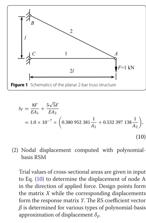
Example 1: Planar 2‑bar Truss Structure The first example is the very simple two-bar truss structure shown in Figure 1.
The given length of bar 1 is 2 l, and the length of bar 2 is √5l. Let l = 1 m.
(1) Analytic expression of nodal displacement
Using the analytic method of structural mechanics, the displacement of node A along the force F direc-tion is as follows:
(6)
γ =YTY− m
i=1
yi
2
/m.
(7) ζmax=max{ζr|r=1, 2,· · ·,S} ,
(8) ζmin=min{ζr|r=1, 2,· · ·,S} ,
(9) ζavg=
M
r=1ζr
S ,
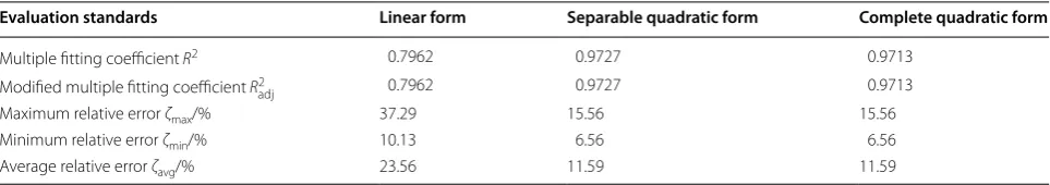
(2) Nodal displacement computed with polynomial-basis RSM
Trial values of cross-sectional areas are given in input to Eq. (10) to determine the displacement of node A in the direction of applied force. Design points form the matrix X while the corresponding displacements form the response matrix Y. The RS coefficient vector β is determined for various types of polynomial-basis approximation of displacement δF.
Linear form:
Separable quadratic form:
Complete quadratic form:
The solving accuracy of polynomial-basis response sur-face method and the selection of the response sursur-face forms are shown in Table 1.
(10) δF= 8F
EA1+
5√5F
EA2
=1.0×10−7×
0.380 952 3811
A1+0.532 397 138
1
A2
,
(11) ˜
y=9.240 1×10⁻⁶−7.047 6×10⁻⁵A1−9.849 3×10⁻⁵A2.
(12) ˜
y=1.373 1×10⁻⁵−2.310 2×10⁻⁴A1
−3.228 6×10⁻⁴A2 +0.002 7A21+0.003 7A
2 2.
(13) ˜
y=1.373 1×10⁻⁵−2.310 2×10⁻⁴A1
−3.228 6×10⁻⁴A2
+0.002 7A21+0.003 7A22−8.456 8×10⁻¹⁸A1A2.
1 2
A B
C l
2l F=1 kN
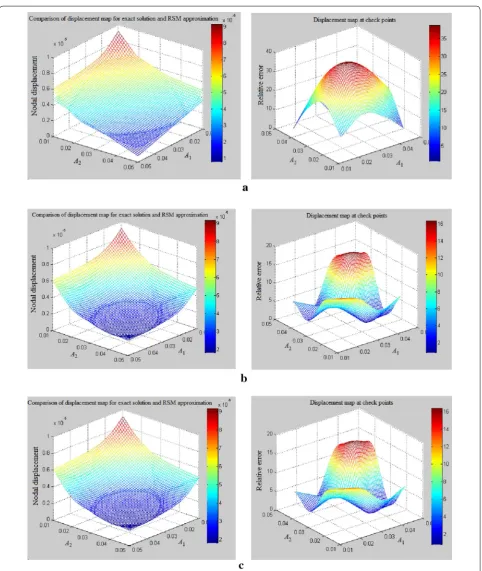
Using the MATLAB software, the surface comparison figure of the analytic value and the response surface esti-mated value and relative error surface figure of the check points are shown in Figure 2.
The accuracy of these RS models is evaluated in Table 1 by means of the performance indicators described in Sec-tion 2.2. Figure 2 compares the variation of nodal displace-ment over the design space determined from the analytical expression (10) or by means of the three RS models. In par-ticular, the MATLAB plots show the displacement map and the relative error map. The following conclusions can be drawn from the results obtained for this example.
(1) The analytical form of the polynomial-basis RS is com-pletely different from the analytic solution (10) which depends on the inverse of cross-sectional areas.
(2) The coefficients of the linear RS model are small. The quadratic RS models are much more accurate than the linear RS model although relative errors at check points remain rather high. Adding cross-terms in the quad-ratic model does not yield substantial improvements.
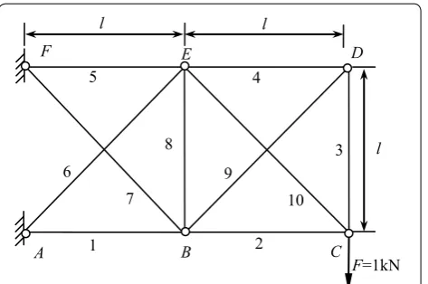
Example 2: Planar 8‑bar Truss Structure In order to check the validity of the above analysis for more compli-cated structures, the statically determinate planar 8-bar truss structure shown in Figure 3 was considered. The length of all bars is 2 m, except for bars 6 and 8 which are 2√2 m long. Loads and kinematic constraints for this
structure are shown in Figure 3.
The analytical solution for the displacement of node C along the direction of applied force F is as follows:
(14) δy=
8F
EA1+
2F
EA2+
2F
EA3+
2F
EA5+
4√2F
EA6 +
2F
EA7+
4√2F
EA8
=1.0×10−7×
0.380952381 1
A1+
0.09523809524
×
1
A2+
1
A3+
1
A5+
1
A7
+0.269340119×
1
A6+
1
A8
Polynomial-basis response surface approximations of displacement give the following results.
Linear form:
Separable quadratic form:
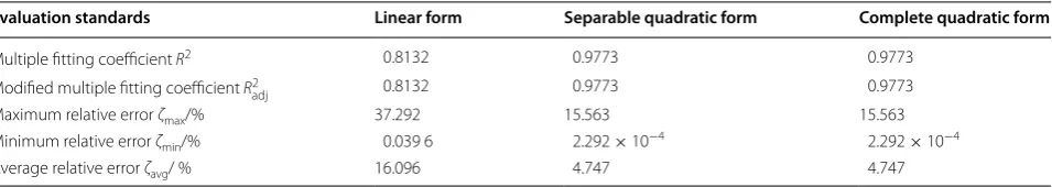
For the sake of brevity, the expression of complete quad-ratic RS is not reported in the article. Performance indi-cators for these RS models are listed in Table 2. The quadratic RS models are again much more accurate than the linear RS model but relative errors at check points remain rather high, thus not satisfying the requirements on overall accuracy. Adding cross-terms in the quadratic model again does not yield substantial improvements. As expected, the analytical form of nodal displacement (14) is completely different from the expressions of RS models.
Since the two truss examples refer to statically deter-minate structures, a statically indeterdeter-minate structure is now analyzed to draw more general conclusions.
Example 3: Planar 6‑bar Truss Structure Figure 4 shows the schematic of a statically indeterminate 6-bar truss structure, in which l is the length and l = 1 m. The displacement to be computed is that of node B along the direction of applied force F.
The accuracy of linear, separable quadratic and full quadratic RS models is listed in Table 3.
The data listed in the table lead to similar conclusions as in the case of statically determinate structures. How-ever, introducing cross-terms in the quadratic RS model
(15) ˜
y=1.315 81×10−5−1.0×10−5×(7.047 6A1+1.761 9 ×(A2+A3+A5+A7) +4.982 8×(A6+A8)).
(16) ˜
y=1.955 2×10⁻⁵−1.0×10−4×(2.310 2A1+5.775 5 ×(A2+A3+A5+A7)+1.633 4×(A6+A8)) +0.002 7×A21+6.689 3×10−
4
×(A22+A 2 3+A
2 5+A
2 7) +0.001 9×(A26+A
2 8).
Table 1 Accuracy of linear, separable and complete quadratic RS models for the 2‑bar truss structure problem
Evaluation standards Linear form Separable quadratic form Complete quadratic form
Multiple fitting coefficient R2 0.7962 0.9727 0.9713
Modified multiple fitting coefficient R2adj 0.7962 0.9727 0.9713
Maximum relative error ζmax/% 37.29 15.56 15.56
Minimum relative error ζmin/% 10.13 6.56 6.56
now yields a more clear improvement over separable quadratic RS model.
The above examples demonstrate that nodal displace-ments of both statically determinate and indeterminate truss structures are multivariate rational functions of cross-sectional areas. This model is totally different from the analytical form of polynomial-basis response surfaces which cannot hence describe correctly the nodal dis-placement field of truss structures.
2.4 Evaluation of the Accuracy of Polynomial‑Basis RSM with Reciprocal Variables
The displacement of a certain node in a given direction computed using Mohr’s theorem can be expressed as
where Nj is the internal force of jth element under the action of true load, Nj0 is the internal force of the jth ele-ment under the action of unit force with the computed displacement direction, lj is the element length, and M is the number of elements.
Let xj=1
Aj, consequently, Eq. (17) can be expressed as
(17)
δi= M
j=1 Nj0Njlj
EAj
,
(18)
δi= n
j=1 Nj0Njlj
E xj.
The most commonly used RS approximation func-tion of nodal displacements of truss structures can be obtained by taking the reciprocal variables xj as design variables and substituting them into Eqs. (1), (2) and (3).
In order to analyze the accuracy of the polynomial-basis response surface method with reciprocal variables, the accuracy analysis is carried out by reusing Example 1‒3 as the examples.
Example 4: Planar 2‑bar Truss Structure For the 2-bar truss structure studied in Example 1, the computing accuracy of polynomial-basis RSM with reciprocal vari-ables is listed in Table 4.
Example 5: Planar 8‑bar Truss Structure For the planar 8-bar truss structure studied in Example 2, accuracy of polynomial-basis RSM with reciprocal variables is listed in Table 5.
Example 6: Planar 6‑bar Truss Structure For the planar 6-bar truss structure studied in Example 3, accuracy of polynomial-basis RSM with reciprocal variables is listed in Table 6.
The following conclusions can be drawn from the results of the above these examples.
4
2
3 7
6
1 5
8
D E
F
A B
C l
l l
F=1kN Figure 3 Schematics of the planar 8‑bar truss structure
Table 2 Accuracy of linear, separable and complete quadratic RS models for the 8‑bar truss structure problem
Evaluation standards Linear form Separable quadratic form Complete quadratic form
Multiple fitting coefficient R2 0.8132 0.9773 0.9773
Modified multiple fitting coefficient R2adj 0.8132 0.9773 0.9773
Maximum relative error ζmax/% 37.292 15.563 15.563
Minimum relative error ζmin/% 0.039 6 2.292 × 10⁻⁴ 2.292 × 10⁻⁴
Average relative error ζavg/ % 16.096 4.747 4.747
1
5
2 6
B
D C
3
4 A
l
l
F=1kN
(1) For the statically determinate structure, the evalua-tion coefficients are very good. The all relative errors are less than 10−10, therefore the approximation accuracy is very high. This is mainly because the pol-ynomial-basis RSM with reciprocal variables equa-tion have a high consistency in the form with the analytic solution, and the response surface equation reflects the true relationship between displacement and design variables.
(2) For the statically indeterminate structure, the approx-imation accuracy is very low. This is mainly because internal forces are changing as the changes of design variables, and these changes don’t be reflected in RSM equation, which lead to the difference in the form between RSM approximation with reciprocal variables and analytic solution. In order to improve the approximation accuracy, a new method of high accuracy response surface should be developed. Table 3 Accuracy of linear, separable and complete quadratic RS models for the 6‑bar truss structure problem
Evaluation standards Linear form Separable quadratic form Complete quadratic form
Multiple fitting coefficient R2 0.8026 0.8991 0.9996
Modified multiple fitting coefficient R2adj 0.8026 0.8990 0.9996
Maximum relative error ζmax/% 28.68 22.66 14.43
Minimum relative error ζmin/% 2.76 3.98 5.01
Average relative error ζavg/% 18.93 11.82 8.96
Table 4 Accuracy of linear, separable and complete quadratic reciprocal variables RSM models for the 2‑bar truss struc‑ ture problem
Evaluation standards Linear form Separable quadratic form Complete quadratic form
Multiple fitting coefficient R2 1 1 1
Modified multiple fitting coefficient R2adj 1 1 1
Maximum relative error ζmax/% 5.78 × 10⁻¹⁴ 1.68 × 10⁻¹² 1.13 × 10⁻¹²
Minimum relative error ζmin/% 1.14 × 10⁻¹⁴ 1.09 × 10⁻¹² 5.22 × 10⁻¹³
Average relative error ζavg/% 3.38 × 10⁻¹⁴ 1.40 × 10⁻¹² 8.21 × 10⁻¹³
Table 5 Accuracy of linear, separable and complete quadratic reciprocal variables RS models for the 8‑bar truss structure problem
Evaluation standards Linear form Separable quadratic form Complete quadratic form
Multiple fitting coefficient R2 1 1 1
Modified multiple fitting coefficient R2adj 1 1 1
Maximum relative error ζmax/% 2.76 × 10⁻¹¹ 2.70 × 10⁻⁹ 4.72 × 10⁻¹¹
Minimum relative error ζmin/% 9.90 × 10⁻¹² 4.15 × 10⁻¹⁴ 5.23 × 10⁻¹³
Average relative error ζavg/% 1.90 × 10⁻¹¹ 6.70 × 10⁻¹⁰ 2.10 × 10⁻¹¹
Table 6 Accuracy of linear, separable and complete quadratic reciprocal variables RS models for the 6‑bar truss structure problem
Evaluation standards Linear form Separable quadratic form Complete quadratic form
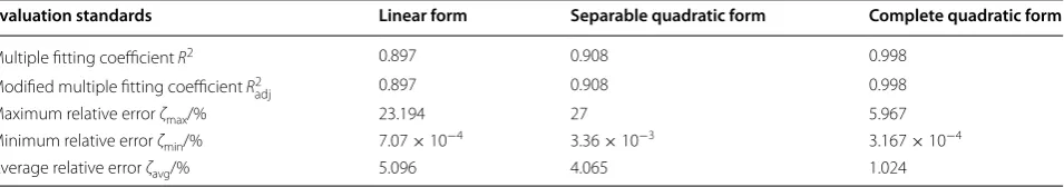
Multiple fitting coefficient R2 0.897 0.908 0.998
Modified multiple fitting coefficient R2adj 0.897 0.908 0.998
Maximum relative error ζmax/% 23.194 27 5.967
Minimum relative error ζmin/% 7.07 × 10⁻⁴ 3.36 × 10⁻³ 3.167 × 10⁻⁴
3 Determination of Nodal Displacements of Truss Structures
According to the finite element method theory, the bal-ance equation is as
The displacement equation is as
Where the inverse matrix can be obtained by the formula as
According to the theory of determinants, the n-order determinant is a number firmed by n2 elements of a
ij.
where τ (j1j2· · ·jn) is the inverted sequence number of natural numbers 1,2,…,n, and
j1···jn is the sum of all per-mutations of natural numbers 1,2,…,n.
Since elements aij of stiffness matrix include products of linear terms corresponding to cross-sectional areas, the determinant can be simplified as
where f(An) is an n-order polynomial of cross-sectional area variables A, and n is the order of the stiffness matrix, equal to the DOF of the structure system.
Elements of the adjoint matrix adjK are polynomials
gij(An−1) which are one order lower than the determi-nant of the stiffness matrix. Thus, the form of the adjoint matrix is
Combining all of the above formulas, it can be obtained the equation to analytically determine nodal displace-ments of truss structures:
Consequently, the displacement of a certain node in a given direction can be expressed as
(19) Kδ=F.
(20) δ=K−1F.
(21) K−1= adjK
|K| .
(22) |K| =
a11 a12 · · · a1n
a21 a22 · · · a2n .
.
. ... ...
an1 an2 · · · ann
= j1···jn
(−1)τ (j1j2···jn)a
1j1a2j2· · ·an jn,
(23) |K| =f(An),
(24) adjK=
g11(An−1) · · · g1n(An−1) ..
. ...
gn1(An−1) · · · gnn(An−1)
.
(25) δ=K−1F= adjK
|K| F.
4 Conjecture about the Determinant Expression of Stiffness Matrix and Elements of Adjoint Matrix
The previous derivation indicate that the determinant of the stiffness matrix of the truss structure and the elements of adjoint matrix involved in the determination of nodal dis-placements are respectively n-order and (n–1)-order poly-nomials. Stiffness matrix determinant is an algebraic sum including n! terms each of which is the product of n factors belonging to different rows and columns. The sign of each term depends on the corresponding inverted sequence number. Therefore, there are at least n! coefficients. Simi-larly, determinants of adjoint matrix elements are algebraic sums of (n–1)! terms each of which corresponds to the product of (n–1) factors belonging to different rows and different columns. The adjoint matrix is an n-order square matrix. Equation (26) implies that 2n! function evaluations must be done. However, if matrix order changes, the num-ber of coefficients also will change in a factorial way. Hence, if the equation order gets large, too many combinations should be considered. Variable linking and relationships between cross-sectional area variables may greatly reduce computational complexity of combinations and multivari-ate rational function response surfaces can be built based on these relationships. The above mentioned relationships will be illustrated by the following examples.
(1) For the 2-bar truss structure considered in Example 1, displacement of node A in the direction of applied load F has the following analytical expression:
where,
(2) For the statically indeterminate 6-bar truss structure considered in Example 3, the analytical expression for the nodal displacement of node B along the direction of applied force F is as follows:
(26) δi= 1
|K|
n
j=1
gij(An−1)Fj =
1
f(An) n
j=1
gij(An−1)Fj.
(27) δAF=
1
|K|
n
j=1
g1j(An−1)Fj=
1
f(A2)g12(A)F,
f(A2)= E
2
50l2
√
5A1A2, g12(A)= E
l
A1
2 + 4√5A2
25
(28) δBF =
1 |K|
n
j=1
g1j(An−1)Fj= 1 f(A5)g33(A
where
The following conjecture can be made from the previ-ous relationships. The determinant of stiffness matrix and the adjoint matrix term entailed in the determination of a certain nodal displacement are polynomials of the same order as the corresponding matrices. Each term of these polynomials is the product of first power terms cor-responding to cross-sectional areas.
where i1�=i2�=i3�= · · · �=i(n−1)�=in.
The number of DOF n is the same as the order
of stiffness matrix; m is the number of design
vari-ables. An are the possible combinations of
cross-sectional areas Ai selected from the set of m design
variables; m1 is the number of these combinations,
namely, m1=Cmn =m!
[(m−n)!n!]. Similarly, An−1 are other possible combinations of cross-sectional areas
Ai; m2 is the number of these combinations, namely,
m2=Cmn−1=m!
[(m−n+1)! ·(n−1)!]; α and β are unknown coefficients to be determined.
The number of terms included in matrix stiffness deter-minant decreases from n! to m!
[(m−n)!n!]; while the number of terms in the corresponding adjoint matrix decreases from (n-1)! to m!
[(m−n+1)! ·(n−1)!] ,
thus reducing the computational cost of the fitting process.
Let′s now consider a statically determinate structure
with m bars and n DOFs. Since there are no
redun-dant bars, it holds m = n. Hence, in Eq. (29), it holds
m1=Cmn =Cnn=1, m2=Cmn−1=Cnn−1=n and the
equation simplifies to
f(A5)= E
5
16l5(2A1A2A3A5A6+2A1A2A4A5A6+A1A3A4A5A6
+A2A3A4A5A6+4 √
2A1A2A3A4A5+4 √
2A1A2A3A4A6),
g33(A4)= E4
16l4(16A1A2A3A4+4
√
2A1A2A3A6+4
√
2A1A2A4A6
+4√2A1A3A4A5+2A1A3A5A6+2A1A4A5A6
+4√2A2A3A4A5+2A2A3A5A6+2A2A4A5A6).
(29)
f(An)= m1
�
i=1
αiAi1Ai2· · ·Ain,
g(An−1)=
m2
�
i=1
βiAi1Ai2· · ·Ai(n−1),
(30)
f(An)=b0A1A2· · ·An,
gij(An−1)=a1A1A2· · ·An−1+a2A1A3· · ·An+ · · · +
aiA1Ai· · ·An+ · · · +anA2A3· · ·An.
By substituting Eq. (30) into Eq. (26), it follows
where Cj=an−j+1/b0.
For statically determinate structures, if the external force P is known, internal forces Nj developed in each bar are constant. If the generalized displacement δi in the direction i is computed using Mohr’s theorem, a unit generalized force Ni0 is applied in the direction i and the corresponding internal forces Nj in each bar also are con-stant. Element lengths lj and cross-sectional areas Aj are constant values as well. Therefore, nodal displacements of a truss structure can be expressed as
where the constant C is equal to Cj=NjNj0lj
E.
The consistency of Eqs. (31) and (32) proves that it may be reasonable to approximate nodal displacements of statically determinate truss structures with multivari-ate rational response surfaces. The following examples will prove the validity of this conclusion also for statically indeterminate trusses.
Example 7: Planar 10‑bar Truss Structure For the pla-nar 10-bar truss structure shown in Figure 5, the general form of the determinant of the stiffness matrix is for this structure is as follows:
The corresponding adjoint matrix element involved in the determination of the displacement of node C in the direction of applied load F is as follows:
(31)
δi=
C1 A1 +
C2
A2 + · · · + Cn
An = n
j=1 Cj
Aj ,
(32)
δi= n
j=1 NjNj0lj
EAj = n
j=1 Cj Aj ,
(33) f(An)= E
8
l8(8A1A10A2A3A4A5A6A8
+8A1A10A2A3A4A5A7A9
+A1A10A2A3A4A6A7A9+ · · ·
+βAaAbAcAdAeAfAgAh+ · · ·).
(34) g67(An−1)= E
7
where {a, b, c, d, e, f, g, h} ∈ {1, 2, 3, 4, 5, 6, 7, 8, 9, 10},
α and β are the unknown coefficients of the products of design variable Ai, and a ≠ b ≠ c ≠ d ≠ e ≠ f ≠ g ≠ h.
Example 8: Spatial 18‑bar Truss Structure For the spa-tial 18-bar truss structure shown in Figure 6, determinant of stiffness matrix is as follows:
The corresponding adjoint matrix element involved in the determination of the displacement of node A in the direction of applied load F is as follows:
where {a, b, c, d, e, f, g, h, i, j, k, l, m, n, o, p, q, r} ∈ {1, 2, 3, 4, 5, 6, 7, 8, 9, 10, 11, 12, 13, 14, 15, 16, 17, 18}, α and β are the unknown coefficients of the products of design vari-able Ai, and a ≠ b ≠ c ≠ d ≠ e ≠ f ≠ g ≠ h ≠ i ≠ j ≠ k ≠
l ≠ m ≠ n ≠ o ≠ p ≠ q ≠ r.
Other examples not documented in this article for the sake of brevity confirm the validity of the conjecture made on the mutual relationship between the stiffness matrix of the truss structure and adjoint matrix elements.
(35) f(An)=E
12
l12 (2175A1A2A17A18A5A9A11A12A15A16A13A14 +76√2A1A17A18A4A5A9A10A12A15A16A11A14
+128√2A1A3A6A8A2A9A10A4A11A12A15A16+ · · · +αAaAbAcAdAeAfAgAhAiAjAkAl+ · · · + · · ·).
(36) g12(An−1)=E
11
l11 (4096 √
2A1A3A6A2A7A17A5A10A11A12A15
+2048A1A3A6A2A7A5A4A11A16A13A14 +768A1A3A6A17A18A5A4A9A10A13A16
+6144√2A1A3A2A7A17A18A5A9A10A11A16+ · · · +αAaAbAcAdAeAfAgAhAiAjAk+ · · ·),
5 Multivariate Rational Response Surface Approximation of Truss Nodal Displacements
Response surface approximation of truss nodal displace-ments can be built as follows:
where αi and βij′ are the RS fitting coefficients to be determined with βij′ = βijFj; m1 and m2, respectively, are the number of terms included in polynomials f(An) and
gij(An−1).
Suitable design points are defined including the cross-sectional areas of the M bars forming the truss. For the generic design “C”, it holds Ak = AkC with k = 1, 2,…, M.
After the displacement δiC corresponding to design points is determined from finite element analysis, Eq. (37) is rewritten as follows:
or
(37) δi=
1 f(An)
n
j=1gij(A
n−1)F
j
=
n
j=1( m2
i=1βijAi1Ai2· · ·Ain−1)Fj m1
i=1αiAi1Ai2· · ·Ain
=
Fj�=0
m2 i=1β
′
ijAi1Ai2· · ·Ain−1 m1
i=1αiAi1Ai2· · ·Ain
,
(38) δCi
m1
i=1 αiACi1A
C i2· · ·ACin
= n
Fj�=0 m2
i=1 βij′AC
i1A
C
i2· · ·ACi(n−1),
(39) δCi
m1
i=1
αiACi1A
C i2· · ·A
C in
−
n
Fj�=0 m2
i=1
β′ijACi1A
C i2· · ·A
C i(n−1)=0. 4
2
3 8
6
1 5
7
D E
F
A B
9
10
C l
l l
F=1kN
Figure 5 Schematics of the planar 10‑bar truss structure
3
1 4 11
7 6
2 5
8
9
10
12
13 14
15 16 17
18
The above expression is a homogeneous equation. Since the ratio between numerator and denominator in Eq. (37) stays the same if both terms are multiplied by the same quantity, RS model coefficients can be normalized with respect to any fitting coefficient. In order to keep general-ity, let us set α1 = 1 and rewrite Eq. (39) as follows:
Selecting M design points (M ≥ m1 + Km2, where K is the number of loads Fj that are not equal to zero), a sys-tem of M linear equations in the unknown coefficients αi and βij′ is obtained:
The determination of these coefficients by solving this system can be done in two ways.
(1) If M > m1 + Km2, the number of design points is larger than the number of unknown coefficients. Solving accuracy is maximized by using the least square method.
(2) If M = m1 + Km2, the number of design points is equal to the number of unknown coefficients and classical linear algebraic solvers can be utilized.
According to best uniform approximation theory, qual-ity of RS approximation improves as the fitting model resembles the real structural response. Since the multi-variate rational RS model developed in this study repro-duces the actual analytical model behind determination of nodal displacements of truss structures, the present model can give results very close to the real structural response of a truss structure.
(40) n
Fj�=0 m2
i=1
βij′ACi1ACi2· · ·ACin−1
−δiC
m1
i=2
αiACi1ACi2· · ·ACin
=δiCACi1.
(41) n � Fj�=0
m2
� i=1
βij′ACi11A
C1
i2· · ·A
C1
i(n−1)−δ C1
i �m1
� i=2
αiAC1
i1A
C1
i2· · ·A
C1
in �
=δC1
i A
C1
i1,
n � Fj�=0
m2
� i=1
βij′ACi12A
C2
i2· · ·A
C2
i(n−1)−δ C2
i �m1
� i=2
αiAC2
i1A
C2
i2· · ·A
C2
in �
=δC2
i A
C2
i1,
. . .
n � Fj�=0
m2
� i=1
βij′ACM i1 A
CM i2 · · ·A
CM i(n−1)−δ
CM i
�m1 � i=2
αiACM i1 A
CM i2 · · ·A
CM in
�
=δCM
i A
CM i1 .
6 Verification of Multivariate Rational RS Model for Truss Displacement Approximation
The accuracy of the multivariate rational response sur-face approximation model developed in this study is verified in some design examples. The cross-sectional area of truss elements is selected as the design variable which can range between 0.01 and 0.05 m2; cross sections of all elements are supposed to be circular. The Young’s modulus is 2.1 × 10¹¹ Pa while Poisson’s ratio is 0.3.
Node displacement is taken as the structural response to be approximated. Value of design variables selected for design points PD is APD,i∈ {0.01, 0.02, 0.03, 0.04, 0.05}
while value of design variables selected for check points PE is APE,i∈ {0.015, 0.025, 0.035, 0.045}.
Example 9: Planar 2‑bar Truss Structure For the truss studied in Example 1, accuracy of multivariate rational RS model is evaluated in Table 7. Figure 7(a) compares the displacement maps corresponding to the true struc-tural response and the approximate model. The relative errors on nodal displacements evaluated at check points are shown in Figure 7(b).
Example 10: Planar 6‑bar Truss Structure The struc-tural layout, kinematic constraints and loads are the same as for Example 3. Table 8 lists the values of performance indicators for the multivariate rational RS model.
Example 11: Planar 12‑bar Truss Structure The pla-nar truss shown in Figure 8 is a statically indeterminate structure constrained by fixed-hinged supports around the edge. There are only two degrees of freedom for this design example. Performance indicators for the multi-variate rational RS model, evaluated with respect to the solution provided by the commercial finite element soft-ware ANSYS, are listed in Table 9.
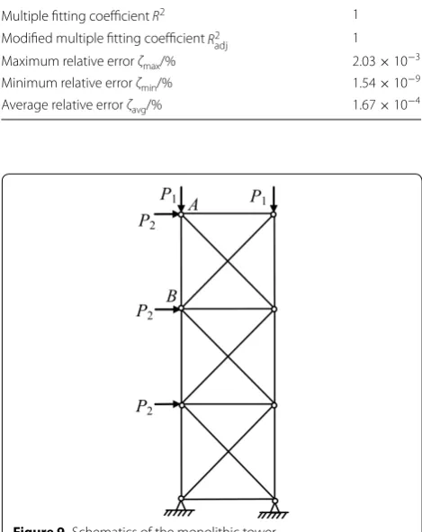
Example 12: Monolithic Tower For the monolithic tower schematized in Figure 9, the lateral load P2 simu-lates the action of the wind while the vertical load P1 simulates the weight of the tower body and other concen-trated loads. Two loading conditions are considered: (i)
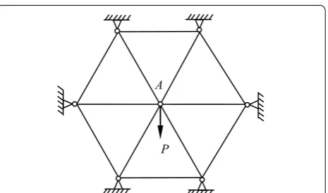
Example 13: Secondary Mirror Supporting Struc‑
ture The secondary mirror supporting structure
sche-matized in Figure 10 is a highly lightweight triangular structure in which six supporting bars form a closed bar system in an end to end way between the primary and secondary mirror plates. The weight of the objects on the top of the supporting structure is equivalent to the con-centrated loads on the three top nodes (see Figure 10). The displacement to be computed is the vertical displace-ment of node A. Performance indicators for the multi-variate rational RS model, evaluated with respect to the solution provided by the commercial finite element soft-ware ANSYS, are listed in Table 11.
It can be seen that relative error between response results obtained by multivariate rational RS approxima-tion and ANSYS is very small for all design examples. Evaluation coefficients are always very high, thus satis-fying engineering requirements. The same conclusion holds true for both statically determinate and indetermi-nate truss structures.
Table 7 Accuracy of multivariate rational RS model for the 2‑bar truss structure problem
Evaluation standards Node A
Multiple fitting coefficient R2 1
Modified multiple fitting coefficient R2
adj 1
Maximum relative error ζmax/% 6.58 × 10⁻¹⁴ Minimum relative error ζmin/% 1.15 × 10⁻¹⁴ Average relative error ζavg/% 2.05 × 10⁻¹⁴
Figure 7 Evaluation of multivariate rational RS approximation accu‑ racy for the 2‑bar structure problem. a Comparison of displacement map for exact solution and RSM approximation. b Displacement error map at check points
Table 8 Accuracy of multivariate rational RS model for the 6‑bar truss structure problem
Evaluation standards Node B
Multiple fitting coefficient R2 1
Modified multiple fitting coefficient R2
adj 1
Maximum relative error ζmax/% 3.63 × 10⁻⁴ Minimum relative error ζmin/% 1.51 × 10⁻⁷ Average relative error ζavg/% 7.46 × 10⁻⁵
P A
7 Conclusions
(1) The polynomial-basis response surface approxi-mation is different from the real function between cross-sectional area and nodal displacement, rela-tive error ranging from 4.747% to 23.56% which does not meet the engineering requirement.
(2) Polynomial-basis RSM with reciprocal variables has a great improvement on the statically determinate structure, with relative errors less than 10−10.
How-ever, for the statically indeterminate structure, the approximation accuracy is still low.
(3) Relationship between the nodal displacement and the cross-sectional area is derived, following the conjecture about the determinant expression of stiffness matrix and elements of adjoint matrix. (4) On the basis of previous conjecture, multivariate
rational response surface approximation of truss nodal displacements is established. The fitting accuracy of both statically determinate structure and statically indeterminate structure is greatly improved, with relative errors less than 10−3.
Table 9 Accuracy of multivariate rational RS model for the 12‑bar truss structure problem
Evaluation standards Node A
Multiple fitting coefficient R2 1
Modified multiple fitting coefficient R2
adj 1
Maximum relative error ζmax/% 2.03 × 10⁻³ Minimum relative error ζmin/% 1.54 × 10⁻⁹ Average relative error ζavg/% 1.67 × 10⁻⁴
A
B P2
P2
P2
P1 P1
Figure 9 Schematics of the monolithic tower
Table 10 Accuracy of multivariate rational RS model for the monolithic tower problem
Evaluation standards Condition 1 Condition 2
Node A Node B Node A Node B
Multiple fitting coefficient R2 1 1 1 1
Modified multiple fitting coefficient R2adj 1 1 1 1
Maximum relative error ζmax/% 3.67 × 10⁻⁴ 3.63 × 10⁻² 4.83 × 10⁻³ 7.08 × 10⁻³ Minimum relative error ζmin/% 2.10 × 10⁻³ 7.30 × 10⁻⁸ 7.65 × 10⁻⁸ 2.76 × 10⁻⁸ Average relative error ζavg/% 5.58 × 10⁻⁴ 2.45 × 10⁻³ 6.72 × 10⁻⁴ 5.18 × 10⁻⁴ Figure 10 Schematics of the secondary mirror supporting structure
Table 11 Accuracy of multivariate rational RS model for the secondary mirror supporting structure problem
Evaluation standards Node A
Multiple fitting coefficient R2 1
Modified multiple fitting coefficient Radj2 1
Authors′ contributions
SC, LJL, MG carried out the multivariate rational response surface approxima‑ tion of nodal displacements of truss structures study. XFJ paticipated in the sequence alignment and drafted the manuscript. And all authors read and approved the final mancuscript.
Author details
1 School of Transportation and Vehicle Engineering, Shandong University
of Technology, Zibo 255049, China. 2 Key Laboratory of Electronic Equipment
Structure Design, Xidian University, Xi′an 710071, China. 3 Shandong Linglong
Tire Co., Ltd., Zhaoyuan 265400, China.
Authors’ Information
Shan Chai, born in 1955, is a professor at School of Transportation and Vehicle Engineering, Shandong University of Technology, China. He received his Ph.D. degree from Dalian University of Technology, China, in 1996. His main research interests include structural optimization, computer aid engineering, vehicle and mechanics dynamics.
Xiang‑Fei Ji, born in 1991, is currently a Ph.D. candidate at Key Laboratory of Electronic Equipment Structure Design, Xidian University, China. His research interests include optimization, noise analysis and control.
Li‑Jun Li, born in 1977, is currently an associate professor at School of Trans-portation and Vehicle Engineering, Shandong University of Technology, China. She received her Ph.D. degree from Shanghai Jiao Tong University, China, in 2005. Her research interests include computer aid engineering, vehicle and mechan‑ ics dynamics, noise analysis and control.
Ming Guo, born in 1989, is currently an engineer at Shandong Linglong Tire Co., Ltd., China. He received his master degree School of Transportation and Vehicle Engineering, Shandong University of Technology, China, in 2006. His main research interests include structural optimization, computer aid engineering.
Acknowledgements
Supported by National Natural Science Foundation of China (Grant No. 5150261), and Shandong Provincial Natural Science Foundation of China (Grant No. ZR2015AM013).
Competing interests
All the authors declare that they have no competing interests.
Ethics approval and consent to participate Not applicable.
Publisher’s Note
Springer Nature remains neutral with regard to jurisdictional claims in pub‑ lished maps and institutional affiliations.
Received: 6 November 2016 Accepted: 16 January 2018
References
1. André I Khuri, Siuli Mukhopadhyay. Response surface methodology. Wiley Interdisciplinary Reviews Computational Statistics, 2010, 2(2): 128‑149. 2. Choon‑Man Jang, Ka‑Ram Choi. Optimal design of splitters attached to
turbo blower impeller by RSM. Journal of Thermal Science, 2012, 21(3): 215‑222.
3. Heng Jiang, Yi‑Sheng Guan, Zhi‑Cheng Qiu, et al. Dynamic and static multi‑objective optimization of a vertical machining center based on response surface method. Journal of Mechanical Engineering, 2011, 47(11): 125‑133. (in Chinese)
4. Hui Lu, De‑Jie Yu, Zhan Xie, et al. Optimization of vehicle disc brakes stability based on response surface method. Journal of Mechanical Engi-neering, 2013, 49(9): 55‑60. (in Chinese)
5. Yong Zhang, Guang‑Yao Li, Zhi‑Hua Zhong. Design optimization on lightweight of full vehicle based on moving least square response surface method. Journal of Mechanical Engineering, 2008, 44(11): 192‑196. (in Chinese)
6. Guang‑Yong Sun, Guang‑Yao Li, Zhi‑Hua Zhong, et al. Optimization design of multi‑objective particle swarm in crashworthiness based on sequential response surface method. Journal of Computational Mechanics, 2009, 45(2): 224‑230. (in Chinese)
7. Chun‑Lin Wang, Hai‑Bo Peng, Jian Ding et al. Optimization for S‑type blade of fire pump based on response surface method. Journal of Mechanical Engineering, 2013, 49(10): 170‑177. (in Chinese)
8. Dong‑Sheng Jia, Guo‑Ping Li, Xiao‑Hui Bai. Structural optimization design of impeller of hydrodynamic coupling based on method of response surface. Coal Mine Machinery, 2010, 31(12): 3‑5. (in Chinese) 9. Xiao‑Jing Wu, Wei‑Wei Zhang, Hua Xiao et al. A Robust Aerodynamic
Design for Airfoil Based on Response Surface Method. Engineering Mechanics, 2015, 32(2): 250‑256. (in Chinese)
10. Wei Wang, Wen‑Hui Fan, Tian‑Qing Chang, et al. Robust collaborative optimization method based on dual‑response surface. Chinese Journal of Computational Mechanics, 2009, 22(2): 169‑176.
11. Min‑Jiu Zhang, Ru‑Jia Gu, Hong‑Shuang Li, et al. Application of response surface method on structural reliability analysis of pin joint in composites.
Journal of Computational Mechanics, 2016, 33(5): 711‑716. (in Chinese) 12. Guang‑Chen Bai, Cheng‑Wei Fei. Distributed collaborative response sur‑
face method for mechanical dynamic assembly reliability design. Chinese Journal of Computational Mechanics, 2013, 26(6): 1160‑1168.
13. Shan Chai, Xiao‑Jiang Shang, Xian‑Yue Gang. Optimization design method and application of engineering structure. Beijing: China Railway Publishing House, 2015. (in Chinese).
14. Yun‑Kang Sui, Hui‑Ping Yu. Improvement of response surface method and its application to engineering optimization. Beijing: Science Press, 2011. (in Chinese)
15. Hong‑Hu Chen, Cheng Tian, Gong‑Gong Peng, et al. Truss structure optimization design based on response surface method. Machine Design and Research, 2016, 32(1): 48‑54. (in Chinese)
16. W J Roux, N Stander, R T Haftka. Response surface approximations for structural optimization. International Journal of Numerical Methods in Engineering, 1998, 42(3): 517‑534.
17. Jun Zhang, Fan Guo. Statistical modification analysis of helical planetary gears based on response surface method and Monte Carlo simulation.
Chinese Journal of Computational Mechanics, 2015, 28(6): 1194‑1203. 18. Wen‑Liang Fan, Chun‑Tao Zhang, Zheng‑Liang Li, et al. An adaptive
response surface method with cross terms. Engineering Mechanics, 2013, 30(4): 68‑72. (in Chinese)
19. M H V Houten, A J G Schoofs, D H V Campen. Response surface tech‑ niques in structural optimization. 1st,WCSMO World Congress of Structural and Multidisciplinary Optimization, Goslar, Germany, 28 May‑2 June, 1995: 89‑95.
20. G Venter, R T Haftka, J H Starnes. Construction of response surface approximations for design optimization. 6th AIAAA/NASA/ISSMO Sympo-sium on Multidisciplinary Analysis and Optimization, Bellevue, Washington, September 4‑6, 1996: 548‑564.
21. Yun‑Kang Sui, Hai‑Bo Bai. Plate shell structural optimization based on central point’s accurate response surface method. Journal of Machine Design, 2005, 22(11): 10‑13. (in Chinese)
22. Nai‑Mei Tang, Yun‑Kang Sui. Membrane structure cross‑sectional optimization based on response surface method. Academic Conference of Chinese Society of Theoretical and Applied Mechanics, Beijing, China, August 26‑28, 2005: 1157‑1158. (in Chinese)
23. Yun‑Kang Sui, Shan‑Po Li. The application of improved RSM in shape optimization of two‑dimension continuum. Engineering Mechanics, 2006, 23(10): 1‑6. (in Chinese)
24. Yan‑Fei Zhao, Yun‑Kang Sui, Hong‑Ling Ye. Optimum design of shell structures with frequency constraints based on response surface meth‑ odology. Journal of Beijing University of Technology, 2006, 32(s1): 19‑23. (in Chinese)