Comparing the speed and accuracy
of approaches to betweenness centrality
approximation
John Matta
1*, Gunes Ercal
1and Koushik Sinha
2Introduction
Many centrality measures exist, utilizing both local and global information for quantify-ing the importance of a node in a network. Local measures such as degree and closeness centrality can be computed in linear time [1], but are limited in their usefulness. Global measures have a much higher time complexity, but have a wider variety of applications. Betweenness centrality [2] is an important global measure based on the shortest paths through an entire network. Given a graph G=(V,E) , where V is a set of vertices and
E ⊂
V
2
is a set of edges, the betweenness centrality of vertex v∈V is defined as
(1)
BC(v)=
s�=v�=t σst(v)
σst , Abstract
Background: Many algorithms require doing a large number of betweenness central-ity calculations quickly, and accommodating this need is an active open research area. There are many different ideas and approaches to speeding up these calculations, and it is difficult to know which approach will work best in practical situations.
Methods: The current study attempts to judge performance of betweenness central-ity approximation algorithms by running them under conditions that practitioners are likely to experience. For several approaches to approximation, we run two tests, clustering and immunization, on identical hardware, along with a process to determine appropriate parameters. This allows an across-the-board comparison of techniques based on the dimensions of speed and accuracy of results.
Results: Overall, the speed of betweenness centrality can be reduced several orders of magnitude by using approximation algorithms. We find that the speeds of individual algorithms can vary widely based on input parameters. The fastest algorithms utilize parallelism, either in the form of multi-core processing or GPUs. Interestingly, getting fast results does not require an expensive GPU.
Conclusions: The methodology presented here can guide the selection of a between-ness centrality approximation algorithm depending on a practitioner’s needs and can also be used to compare new methods to existing ones.
Keywords: Betweenness centrality, Approximation algorithms, GPU algorithms
Open Access
© The Author(s) 2019. This article is distributed under the terms of the Creative Commons Attribution 4.0 International License (http://creat iveco mmons .org/licen ses/by/4.0/), which permits unrestricted use, distribution, and reproduction in any medium, provided you give appropriate credit to the original author(s) and the source, provide a link to the Creative Commons license, and indicate if changes were made.
RESEARCH
*Correspondence: [email protected]
1 Southern Illinois University Edwardsville, Edwardsville, IL, USA
where σst is the number of shortest paths from node s to node t, and σst(v) is the number
of those paths that pass through vertex v.
Betweenness centrality has been applied to problems as diverse as cancer diagnosis [3], network flow [4], and the measurement of influence in social networks [5]. There are many applications involving a large number of betweenness centrality calculations, such as power grid contingency analysis [6] (which is so computationally intensive that it must be done on a supercomputer), Girvan–Newman community detection [7], net-work routing [8], skill characterization in artificial intelligence [9], analysis of terrorist networks [10], node-based resilience clustering [11], and the modeling of immunization strategies [12]. In these applications, the vertex with the highest betweenness centrality must be determined for a continually changing graph O(n) times.
The most efficient known algorithm for calculating exact betweenness centralities is a faster algorithm by Brandes [13]. For unweighted graphs, this algorithm is based on a modification of breadth-first search (BFS) and can calculate the betweenness central-ity of every node in a graph with a time complexcentral-ity of O(|V||E|). Many algorithms used in the biological and social sciences, such as those mentioned above, rely on repeatedly calculating betweenness centrality for every node in a network. The relevant networks examined, such as online social networks, can become arbitrarily large, making Brandes’ algorithm impractical for many realistic scenarios. Therefore, the problem of perform-ing a large number of betweenness centrality calculations efficiently is an active open research area [14] to which this work contributes.
We wish to compare different ways of decreasing the execution time of the above algo-rithms, and both speed and accuracy are important in the assessment of outcomes. Sim-ply comparing the results of approximate betweenness centralities to the true values is not necessarily useful for several reasons. First, several of the aforementioned algorithms use betweenness centrality as a measure of relative importance with which to rank ver-tices, and only the correct ranking is required. An approximation that produces some incorrect values, but preserves the correct ranking will perform just as well as exact cal-culations. Second, for some of the algorithms, even the exact centrality ordering is not critical. For example, it is noted in works such as [15, 16] that only the top or top k verti-ces with the highest betweenness centrality are required. In light of such considerations, approximation algorithms for betweenness centrality that consistently and efficiently discover the highest betweenness node or nodes may be more useful than slower tradi-tional methods computing the betweenness centrality for every node exactly.
are sufficiently accurate and fast for the important applications considered. For example, most methods use parameters which control the trade-off between speed and accuracy. Results in [17] are based on the use of only one set of parameters, while our work follows a methodical process which yields insight into the process of finding and using the best parameters given a preferred outcome.
The present work is an extension of the conference paper A Comparison of Approaches to Computing Betweenness Centrality for Large Graphs [25]. Whereas the previous paper compared only two approaches to increasing the speed of a large number of between-ness centrality calculations, this paper compares many different approaches: eight are fully tested, and experiences with several others are reported upon. The previous paper used a clustering test as the benchmark for comparison. Here we add a second bench-mark, a test based on the immunization problem. A third addition is the comparison of our results to [17]. While [17] is an important related work, we come to very differ-ent conclusions, and the reasons for the differences are analyzed. Finally, because the trade-off between speed and accuracy of approximation methods is determined by user-supplied parameters, this paper gives detailed notes on parameter selection meant to be useful to practitioners.
The rest of the paper is organized as follows. “Background” discusses research in the area of betweenness centrality calculation and provides a useful survey of many different heuristic and approximation methods. “Methods” describes and justifies the tests and graphs used, and the process of carrying out the experiments. “Experimental results” describes individual results for ten different estimation techniques and summarizes per-formance based on both speed and accuracy. A description of each algorithm including its time complexity is given in this section. Finally, “Conclusion” contains a brief sum-mary of the paper.
Background
Attempts to increase the speed of betweenness centrality calculations go back at least to Brandes’s original faster algorithm in 2001 [13]. Brandes’s paper notably establishes a time complexity for exact calculation of O(|V||E|) (for unweighted graphs) against which many other algorithms are compared. Brandes is also known for his paper on variants of betweenness centrality, which provides ideas for efficient implementations [26].
Betweenness centrality is a shortest-paths based measure, and computing it involves solving a single-source shortest paths (SSSP) problem. One heuristic strategy for speed-ing the overall computation is to solve the SSSP problem for a smaller set of vertices. Brandes and Pich’s 2007 work (hereafter referred to as Brandes2007) creates estimates that “are based on a restricted number of SSSP computations from a set of selected piv-ots” [18]. The idea of using a sample, based on an earlier technique for speeding close-ness centrality calculations [27], is tested using different sampling strategies, such as uniformly at random, random proportional to degree, and maximizing/minimizing dis-tances from previous pivots. It is determined that a randomly chosen sample gives best results.
varies with the information obtained from each sample.” For example, a vertex whose neighbors induce a clique has betweenness centrality of zero, and its inclusion in the sample does not provide much information. Geisberger, Sanders and Schultes develop a method termed Better Approximation in [21] (Geisberger2008), in which the process for selecting the pivot nodes is improved. To further increase speed, if an arbitrary number k of vertices is selected, the algorithm can be parallelized for up to k processors. The overall idea of sampling is generalized by Chehreghani in [28], where a framework is given for using different sampling techniques, and a strategy for choosing sampling tech-niques that minimize error is discussed. Further discussion of a large number of sam-pling strategies can be found in [29].
Riondato and Kornaropoulos introduce a different idea for sampling in [20] (Rion-dato2016). In this sampling algorithm, betweenness centrality computations are based not on pivots as in Bader2007 and Brandes2007, but on a predetermined number of samples of node pairs. This fixed sample size results in faster computation with the same probabilistic guarantees on the quality of the approximation. Riondato and Upfall have another technique, called ABRA, that uses Rademacher averages to estimate between-ness centrality [22].
KADABRA (the ADaptive Algorithm for Betweenness via Random Approxima-tion) is described by Borassi and Natale in [30] (Borassi2016). With KADABRA speed is achieved by changing the way breadth-first search is performed and by taking a dif-ferent approach to sampling. The use of parallelization also helps to make it very fast. In addition to computing betweenness centrality for every vertex, the algorithm can be configured to compute the set of the k most-central vertices. This will turn out to be an important property that gives the algorithm great speed with applicable applications. Along these same lines, work by Mumtaz and Wang focuses on identifying the top-k influential nodes in networks using an estimation technique which is based on progres-sive sampling with early stopping conditions [31].
In general, the time complexity of the sampling algorithms (such as described above) is based on the O(|V||E|) time complexity of Brandes’ algorithm, but is proportional to the number of samples. The algorithms therefore have a practical time complexity of O(k|E|) where k is the number of samples used. The fact that all time complexities are the same makes the actual performance of the algorithms difficult to judge and says nothing about the accuracy obtained.
do “hierarchical decomposition” of a graph. These strategies speed computation by shrinking the size of the graph that must be computed. Chehreghani et al. [37] have an algorithm that combines both graph reduction and sampling techniques, although it applies only to directed graphs.
As with the sampling algorithms, the time complexity for the network-reducing algorithms is, in the worst case, the same O(|V||E|) as computing the entire graph, and performance must be measured empirically.
The calculation of many elements of betweenness centrality can be run in parallel, and this is a widely attempted strategy. Sariyüce et al. have developed algorithms for use with heterogeneous architectures, by which they mean using multiple CPU cores and a GPU concurrently. Their algorithm is called “gpuBC” [38], and they borrow ideas from BADIOS, as well as introducing new ideas specific to GPU architecture.
In addition to [21, 30, 38], ideas for distributed methods include those by Wang and Tang [39], Shi and Zhang [40], and works by David Bader with Adam McLaughlin [41] and other authors [42, 43]. McLaughlin and Bader introduce Hybrid-BC in [41] (McLaughlin2014). The term hybrid refers to the use of a combination of approaches. The first approach is edge parallel, where each edge is assigned to a different thread. The second approach is called work-efficient, where each vertex is handled by a sepa-rate thread in a manner that minimizes redundant or wasted work. At each iteration, either an edge-parallel or work-efficient algorithm is chosen depending on the over-all structure of the graph. Other algorithms exploiting extreme parover-allelism involving multiple GPUs are explored by Bernaschi et al. [44, 45]. In [46], Ostrowski explores using big-data techniques such as map reduce to decompose a graph resulting in faster computations.
Some ideas are radically different and offer unique perspectives on the problem of speeding betweenness centrality calculations. Yoshida’s [1] paper on adaptive betweenness centrality is such a work. The term adaptive betweenness centrality is defined in [12] and refers to computing betweenness centrality for a succession of vertices “without considering the shortest paths that have been taken into account by already-chosen vertices” [1]. In effect, adaptive betweenness centrality means that once the vertex with top betweenness centrality is chosen, it is removed from the net-work along with its adjacent vertices. Subsequent calculations of betweenness central-ity are calculated based on this newly configured network. This description matches exactly the method of calculating used in our benchmark problems. Like Yoshida’s method, the HEDGE algorithm introduced in [47] works with evolving networks and has provable bounds on the accuracy of the approximation. An additional algorithm with applicability to dynamic networks is described in [48].
One last speed enhancing strategy is to substitute a different measure that is easier to compute, but has results that correlate with betweenness centrality. This has been attempted using such measures as Katz centrality [49], closeness centrality [1], κ-path centrality [50], and routing betweenness centrality [51]. A variation on this strategy is to use local measures to estimate global betweenness centralities [52].
1 Compute fewer shortest paths, by extrapolating information from pivots, or other-wise limiting the number of SSSP problems solved [18–22].
2 Partition the graph in a way that preserves betweenness centralities, but allows them to be computed on a smaller vertex set [33, 34, 38].
3 Use multiple cores or a GPU to compute shortest paths simultaneously, or otherwise parallelize an algorithm [21, 30, 38, 41].
4 Use an adaptive approach, which, instead of removing nodes and recalculating in a loop, attempts to calculate directly the succession of top betweenness centrality ver-tices, taking into account the removal of previous vertices [1].
5 Identify influential nodes using easier to compute measures that are correlated with betweenness centrality such as coverage centrality [1], or κ-path centrality [50].
Methods
The goal of this work is to compare the speed and accuracy of several different approximation algorithms for betweenness centrality in the context of important applications. For each algorithm, we attempt to perform two tests. First, a cluster-ing test is performed on a series of six 10,000-node graphs. Parameters are chosen strategically to balance speed and accuracy. If results are promising, we continue the clustering test with six 100,000-node graphs. Third, we run the immunization test on three popular graphs from SNAP [53]: email-enron, p2p-Gnutella31, and soc-sign-epinions. If results are exceptional, we run the immunization test on a fourth graph, web-Google. In this section we describe the clustering test, the immunization test, the graphs used, and the strategy for choosing parameters.
The scope of the experiment
The clustering test
The first evaluation of approximation approaches is conducted with the clustering test, which uses a graph clustering methodology called node-based resilience measure cluster-ing (NBR-Clust). A specific variant of NBR-Clust is first discussed in [54], and the full framework is defined in [11]. As implied by the name, node-based resilience clustering takes a resilience measureR(G) as a functional parameter computed on the input graph G. Every node-based resilience measure operates by computing a limited size attack setS of vertices whose removal causes substantial disruption to the graph with respect to the resulting connected component size distribution. NBR-Clust takes the resulting com-ponents to be the foundational clusters, and completes the clustering of the input graph G by subsequently adding each attack set node in S to its appropriately chosen adjacent cluster. The description of the NBR-Clust framework follows.
The NBR-Clust clustering framework
1 Approximate a resilience measure R(G) with acceptable accuracy and return the cor-responding attack set S whose removal results in some number ( ≥2 ) of candidate clusters. In these experiments we will use the resilience measure integrity [55] as R(G).
2 Create G′=G\ {S} , which must consist of two or more candidate clusters.
3 Adjust the number of clusters. Datasets used in this experiment come with automati-cally generated ground truth data, including the number of clusters the graph con-tains. If more clusters have been obtained than that indicated by the ground truth data, clusters are joined based on their adjacencies. If there are not enough clusters, choose the least resilient of the clusters (based on the resilience measure R) and repeat steps 1 and 2 on that cluster. Continue until the correct number of clusters is obtained.
4 Assign attack set nodes to clusters.
The dependence of NBR-Clust on betweenness centrality calculations, in turn, hinges upon the calculation of the node-based resilience measure R. Many resilience measures exist across a large number of applications. One example is the controllability of a com-plex network [56, 57], which uses control theory to determine a set of driver nodes that are capable of controlling the network and is applicable to static networks as well as net-works with changing topologies [58, 59]. A specific measure is control centrality which quantifies a node’s ability to perform as a driver. Such resilience measures can be used as R(G) with the NBR-Clust framework. In [58], it is noted that the control centrality of a node is not determined by its degree or betweenness centrality, but by other factors. We are looking to measure the speed of calculating betweenness centrality, and therefore do not use such measures in our experiments.
particularly on the most relevant measures such as integrity, VAT, and tenacity. Integrity quantifies resilience by measuring the largest connected component after removal of an attack set. Integrity is defined as
where S is an attack set and Cmax(V −S) is the largest connected component in V−S . Because integrity is a function of the largest connected component size distribution, it shares a similarity with the immunization problem and well-studied methods of maxi-mizing results on both problems use betweenness centrality.
With Greedy-BC, the highest betweenness vertex is calculated and removed from the graph. This process is repeated until all nodes have been removed, and the attack set whose removal results in the smallest resilience measure value is returned. Given a resil-ience measure R, the resilience measure of a specific graph G denoted by R(G), and the resilience measure of a specific graph G with attack set S removed denoted by R(S, G), the steps of Greedy-BC are as follows:
The Greedy-BC heuristic
1 Rmin=R(G) , Smin= {} 2 repeat |V| times
3 v=argmaxv∈VBC(V) 4 G=G\ {v} and S=S∪ {v}
5 if R(S,G) <Rmin then Rmin=R(S,G) and Smin=S 6 return Smin.
Amongst the various resilience measures considered, integrity was found to be particu-larly useful with respect to the application to clustering in NBR-Clust due to the higher accuracy and one-step clustering it provides when the number of clusters is not known a priori [11]. Therefore, the resilience measure we use here with NBR-Clust is integrity [55]. Here, I(G) from Eq. 2 will be the resilience measure called for by R(G)
NBR-Clust is a good test case for algorithms that speed up betweenness centrality cal-culations because it shares many of the properties of practical problems that practition-ers face. First, the exact values being calculated are not important. The algorithm does not use the exact value, except to determine the highest ranking vertex. Therefore, it is the ranking of vertices that is important, and small variations of ranking do not change the result. Second, because a large number of calculations are required (conceivably O(n2) betweenness centralities must be calculated), scalability is tested. Third, the use-fulness of the results can be judged by the accuracy of the resulting clustering, which allows for presentation of results along two axes of speed and accuracy. Because of its similarities to many algorithms, results from NBR-Clust can be generalized to other algorithms that also rely on a large number of betweenness centrality calculations.
One limitation of the clustering test is that the datasets used require a ground truth against which accuracy results can be determined. This limits the types of data that can be used. In this work, we use generated datasets with meaningful ground truth data. We note that, to achieve high accuracy, the clustering test must match a particular predeter-mined outcome, confirming the difficulty of this test.
(2)
I(G)=min
The immunization test
The immunization problem is well known and well studied in the complex networks lit-erature, with applications to diffusion of information [67], identification of important nodes [68], and also to the spread of disease and computer viruses [69]. The immuniza-tion problem involves attacking a network by removing vertices, presumably in the order most likely to cause damage to the network. The problem is made more difficult by limit-ing the number of nodes that can be attacked. The success of the attack is measured by the size of the largest remaining component, also called the giant component.1 There are several well-known strategies for choosing the attack order for the immunization prob-lem. Four of the strategies detailed in [12] are as follows:
i. Select vertices in order of decreasing degree in the original graph and remove ver-tices in that order.
ii. Use an adaptive strategy which involves selecting the highest degree vertex in a graph, removing it, selecting the highest degree vertex in the newly configured graph, and continuing in that fashion.
iii. Select vertices in order of decreasing betweenness centrality in the original graph and remove vertices in that order.
iv. Use an adaptive strategy which involves selecting the highest betweenness central-ity vertex in a graph, removing it, selecting the highest degree vertex in the newly configured graph, and continuing in that fashion.
When the immunization test is conducted in this paper, the adaptive betweenness strategy (strategy iv above) is used to remove nodes from the network until either (1) all nodes have been removed, (2) some predetermined number of nodes have been removed, or (3) the betweenness centralities of the remaining nodes are all zero. Obvi-ously, if all nodes are removed the largest connected component will be zero. We are more interested in seeing if removing smaller numbers of nodes can result in small com-ponents. Therefore, our results show the maximum component size after a predeter-mined number of removals, usually 10% of the nodes in the network.
Graphs used with the clustering test
There are many generative models for graphs, such as Erdös–Rényi random graphs, the planted l-partition model [70], the Gaussian random partition generator [71], and the LFR benchmark network [72]. We test using the LFR benchmark because it is con-sidered state of the art [73] and was created specifically to test community detection algorithms. The LFR Net can be generated based on several parameters, such as mini-mum and maximini-mum cluster size and average and maximini-mum degree and mixing factor. The mixing factor controls the percentage of edges that leave a cluster, also called boundary edges. A higher mixing factor means less tightly bound clusters that are more difficult to detect. One strength of the LFR model is that it accounts for “hetero-geneity in the distributions of node degrees and community sizes” [72], and it is often
used to generate scale-free graphs. We controlled both the degree and the community sizes as described below to keep most graph properties constant while varying mixing factor, and our graphs are not scale free. The graphs are generated according to the following sequence, which is described more fully in [72, 73].
1 A sequence of community sizes is extracted. This is done randomly, although it is controlled by parameters specifying minimum and maximum community sizes. 2 Each vertex i of a community is assigned an internal degree of (1−µ)di , where di is
the degree of vertex i, and µ is the previously described mixing factor. The degree is chosen randomly, although it is subject to parameters controlling its minimum and maximum values. The node is considered to have (1−µ)di stubs, where a stub is a potential edge.
3 Stubs of vertices of the same community are randomly attached until all stubs are used.
4 Each vertex i receives µdi additional stubs that are randomly attached to vertices of different communities, until all stubs are used.
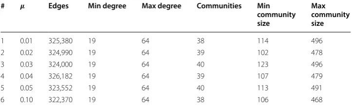
Twelve LFR network graphs are used with the clustering test. Half have 10,000 nodes and half have 100,000 nodes. All graphs are generated randomly, to have approxi-mately 40 communities. The six 10,000-node graphs are generated to have degree dis-tributions from 19 to 64 and community sizes from 100 to 500. Based on extensive experimentation, it was discovered that the mixing factor parameter, denoted µ , had the greatest influence on the ease of clusterability of a graph. Our graphs have mixing factors µ ranging from 0.01 to 0.1. Complete details are given in Table 1.
The 10,000-node graphs 1 through 6 keep properties such as degree structure and average community size constant while changing µ . This allows a test based on clus-tering difficulty without complicating factors such as number of edges (which would require more computation time in edge-based sampling methods). Most of the approximation methods tested use parameters which control the trade-off between speed and accuracy. It is anticipated that succeeding in the clustering test will require much less accuracy for Graph 1 than for Graph 6. Therefore, Graph 1 was used as a baseline accuracy test. It was expected that as accuracy parameters were increased, graphs 2 through 5 would become clusterable, with Graph 6 being the ultimate test. It is noted that Graph 6 is much more difficult to cluster than the first five.
Table 1 10,000-node randomly generated LFR nets used
# µ Edges Min degree Max degree Communities Min community size
Max community size
1 0.01 325,380 19 64 38 114 496
2 0.02 324,990 19 64 39 102 478
3 0.03 324,000 19 64 40 123 496
4 0.04 326,182 19 64 39 107 479
5 0.05 323,552 19 64 40 113 491
A second series of LFR networks with 100,000 nodes was also generated. Details for these graphs are presented in Table 2. The six graphs can best be viewed as two series of three graphs. Graphs 1–3 are characterized by low average degree and low number of edges. They are in order of increasing difficulty. With approximation methods that are based on the number of edges, these graphs should be substantially faster to cluster than graphs 4–6, which have three times as many edges. This gives an effective test of the scalability of the algorithms. To test the power of mixing factor µ over clusterability, graphs 1–3 and 4–6 represent independent progressions of mixing factor. There should be cases where an accuracy parameter setting will fail to cluster Graph 3 but will succeed in clustering Graph 4. However, Graph 4 may take longer because of its larger number of edges. With the largest mixing factor, and a large number of edges, Graph 6 is the most difficult to cluster on all counts. Our goal in setting parameters was to find a combina-tion that would cluster Graph 6 with at least 90% accuracy, although that did not always happen.
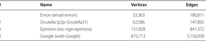
Graphs used with the immunization test
For the immunization test, we used four graphs taken from the SNAP repository [53]. Their information is shown in Table 3.
Choosing parameters
The approximation methods use parameters to control the trade-off between speed and accuracy. For each method that was evaluated, we followed a structured process to find an optimal speed/accuracy trade-off. The steps followed are listed below:
1 We took note of suggested parameters in the source papers, particularly parameters that the authors had used in their own experiments.
Table 2 100,000-node randomly generated LFR nets used
# µ Edges Min degree Max degree Communities Min community size
Max community size
1 0.001 275,542 2 16 36 1026 4567
2 0.003 275,894 3 15 38 1083 4705
3 0.005 275,270 3 15 40 1024 4992
4 0.001 828,375 10 32 37 1100 5566
5 0.005 825,222 10 32 42 1118 4703
6 0.010 826,895 10 32 39 1111 4956
Table 3 Graphs used in the immunization test
# Name Vertices Edges
1 Enron (email-enron) 33,363 180,811
2 Gnutella (p2p-Gnutella31) 62,586 147,892
3 Epinions (soc-sign-epinions) 131,828 841,372
2 We attempted to use parameters discovered in step 1 to cluster the 10,000-node Graph 1, hoping to obtain results of 100% accuracy. If the graph was not clustered to 100% accuracy, we changed the parameters to increase accuracy. This process was repeated until an appropriate setting was found. Often, these parameters successfully clustered graphs 1–6, with varying degrees of accuracy. If possible, we tried to find the fastest setting that gave 100% accuracy with Graph 1.
3 Having found the minimum accuracy settings, we increased the accuracy parameter until Graph 6 was clustered with at least 90% accuracy (although we could not always achieve this in a reasonable time).
4 For comparison, we chose a parameter setting between the settings discovered in steps 2 and 3. We ran the clustering test for all six graphs for all three parameter set-tings.
5 Moving to the 100,000-node graphs, we tried the same settings used for the 10,000-node graphs. The most common problem was that the maximum accuracy setting for the 10,000-node graphs was very slow when used with the 100,000-node graphs. In that case, we tried slightly faster/less accurate settings. In all cases, we tried to find a setting that would cluster 100,000-node Graph 6 with at least 90% accuracy. If that did not succeed, we tried to find a setting where the clustering for Graph 6 at least did not fail. Preliminary work for this paper appeared in [25], and those timings were used as an indication of what should be considered reasonable.
Experimental results
The goal of the experiments is to reproduce the steps a practitioner with a real problem to solve might take to use one of the approximation algorithms, although under more controlled circumstances. In real life, exact calculations of graphs of tens of thousands of nodes are going to take days to run, at least with current, readily available technology. For example, executing the clustering test with 10,000-node Graph 6 took approximately 48 h using Brandes’s exact faster algorithm [13]. We did not have access to a supercom-puter and assume many practitioners do not.
All experiments were conducted on two identical computers. Each had an Intel i7-7700K CPU running at 4.20 GHz with four cores and eight logical processors, and 16 GB ram. Computers also had Nvidia GPU cards, which will be described later. We attempted to use many different betweenness centrality approximation methods, com-piled from a variety of sources, and code from the original authors was used where avail-able. All implementations of algorithms used are available from documented public sources. All were written in C++ (or CUDA and C++) and compiled to optimize speed.
Overall results
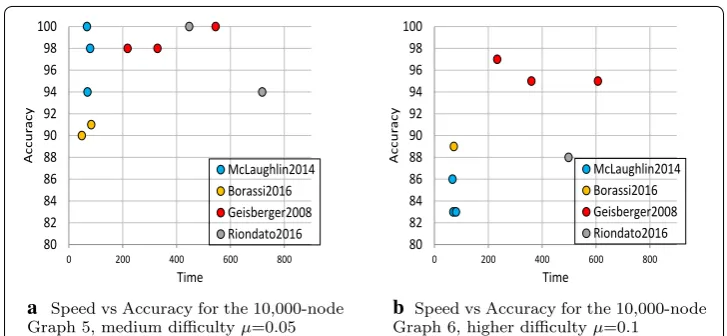
slight gain in speed at the cost of some accuracy, and Geisberger2008 gives consistently good accuracy, but takes more than twice as long. For the more difficult µ=0.1 graphs shown in Fig. 1a, Borassi2016 matches McLaughlin2014 in speed, and in one case beats it in accuracy as well. Two additional runs of the Borassi2016 algorithm (detailed with all runs in Table 18) with speed of 62, accuracy 50% and speed of 50, accuracy 44% did not have high enough accuracy to be shown in Fig. 1b.
The overall clustering test results for 100,000-node graphs are shown in Fig. 2. Results for the sparse-edge Graph 3 are shown in Fig. 2a and for the denser Graph 6 in Fig. 2b. The 100,000-node clustering test is a good indication of the scalability of the algorithms. Note that on the most difficult examples, the Riondato2016 algorithm has dropped off the chart. On the less dense Graph 3, Borassi2016 performs best, both in terms of speed and accuracy. On the denser Graph 6, McLaughlin2014 is the most consistent
80 82 84 86 88 90 92 94 96 98 100
0 200 400 600 800
yc ar uc c A Time McLaughlin2014 Borassi2016 Geisberger2008 Riondato2016
a Speed vs Accuracy for the 10,000-node Graph 5, medium difficultyµ=0.05
80 82 84 86 88 90 92 94 96 98 100
0 200 400 600 800
yc ar uc c A Time McLaughlin2014 Borassi2016 Geisberger2008 Riondato2016
b Speed vs Accuracy for the 10,000-node Graph 6, higher difficultyµ=0.1 Fig. 1 Best performing algorithms for the clustering test on 10,000-node graphs. These results represent optimal conditions. McLaughlin2014 is run using an Nvidia Titan V GPU, and Borassi2016 is configured to return five betweenness centralities at one time
70 75 80 85 90 95 100
0 5000 10000 15000
yc ar uc c A Time McLaughlin2014 Borassi2016 Geisberger2008 Riondato2016
a Speed vs Accuracy for the 100,000-node Graph 3, medium difficulty µ=.005 µ=.005 70 75 80 85 90 95 100
0 5000 10000 15000
yc ar uc c A Time McLaughlin2014 Borassi2016 Geisberger2008
b Speed vs Accuracy for the 100,000-node Graph 6, higher difficulty µ=.01 graph
combination of speed and accuracy, although again some accuracy can be traded for gains in speed with Borassi2016. In both cases, Geisberger2008 is slower but with con-sistently high accuracy.
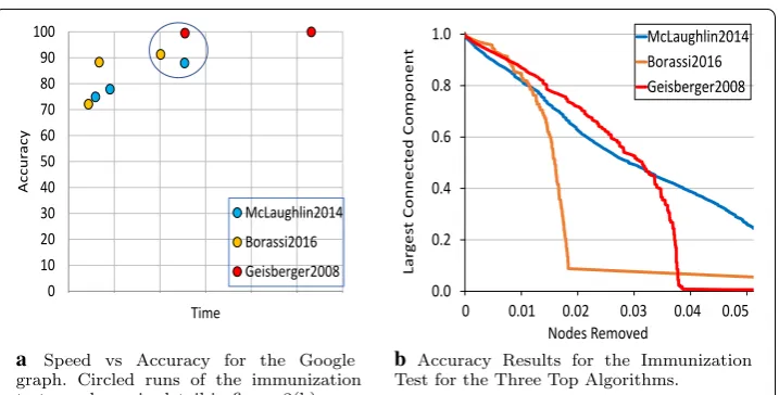
Because of the exceptional performance of McLaughlin2014, Borassi2016 and Geis-berger2008, we tested each further for scalability using the immunization test on the Google dataset, which has 875,713 nodes and over 5 million edges. Results are shown in Fig. 3. Borassi2016 performs very well here, having the best speed, and also the best speed/accuracy combination. McLaughlin2014 was run on an Nvidia Titan V GPU, and performed well with speed, but had trouble achieving accuracy. Results from the cir-cled runs in Fig. 3a, which are shown in Fig. 3b, show that for quick results Borassi2016 performs best. Borassi2016 removes less than 2% of nodes to achieve a smallest cluster of approximately 1%. Geisberger2008 requires attacking almost twice as many nodes to achieve the same results. McLaughlin2014 never achieves the dramatic drop of the other two, and only achieves a smallest component size of 12% in roughly the same amount of time.
Individual algorithm and parameter selection results
Following is a list of tested algorithms. For each algorithm we describe the parameters, show the parameters selected, and, to the extent available, display the results of the clus-tering and immunization tests. All results include a time component, which is given in seconds. Hopefully, this will aid the practitioner in selecting parameters given graph size, available time, and desired performance. We understand that many algorithms are relevant because they contain important new ideas, and that all algorithms do not need to be fastest. We also understand that sometimes those algorithms and ideas will later be incorporated into new algorithms that will surpass previous algorithms in speed or accuracy. All of the algorithms below have made important contributions to the under-standing of the mechanics of calculating betweenness centrality. We test them for speed, although a slower speed does not diminish their importance or usefulness.
0 10 20 30 40 50 60 70 80 90 100
yc
ar
uc
c
A
Time
McLaughlin2014 Borassi2016 Geisberger2008
a Speed vs Accuracy for the Google graph. Circled runs of the immunization test are shown in detail in figure 3(b).
0.0 0.2 0.4 0.6 0.8 1.0
tn
e
n
o
p
m
o
C
de
tc
e
n
n
o
C
ts
eg
ra
L
Nodes Removed
McLaughlin2014 Borassi2016 Geisberger2008
0 0.01 0.02 0.03 0.04 0.05
b Accuracy Results for the Immunization Test for the Three Top Algorithms.
Brandes and Pich 2007 (Brandes2007)
This algorithm is taken from [18], and we used code from [17] to run it. The algo-rithm uses a heuristic: shortest paths are calculated for a group of samples, called pivots, instead of for all nodes in the graph. The paper states that the ultimate result would be that “the results obtained by solving an SSSP from every pivot are representa-tive for solving it from every vertex in V” [18]. They test several different strategies for selecting the pivots, and find that uniform random selection works best. The algorithm tested here uses uniform random selection. The worst-case time complexity of this approach is O(|V||E|). The speedup is directly proportional to the number of pivots, giv-ing a practical time complexity of O(k|E|) where k is the number of pivots. Results are shown in Table 4. For the 10,000-node graphs, 50 samples gave good results on Graph 1 and Graph 2, but accuracies fell for the remaining graphs. Note that 200 samples were required to obtain uniformly high accuracies, and even then did not meet 90% for Graph 6. The 100,000-node graphs got good results with only 25 samples. The 10- and 50-sam-ple results are shown mostly to demonstrate speed. Note that with Graph 3, doubling the number of samples roughly doubles the amount of time required.
It is useful to compare these results to the Bader2007 algorithm (shown in the next section in Table 7). Note that on the 10,000-node graphs, Brandes2007 takes some-times twice or even three some-times as long as Bader2007, even though the latter algorithm required a larger number of samples. With the 100,000-node graphs, Brandes2007 was able to cluster Graph 6 with 200 samples, while Bader2007 required 250 samples. None-theless, the time for Bader2007 is shorter and the accuracy higher. Both algorithms have the same theoretical time complexity, making the large difference in running times an interesting result.
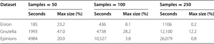
Numerical results for the immunization test are shown in Table 5. Brandes2007 does very well with 100 and 250 samples. The time for the large Epinions dataset with 100 Table 4 Brandes2007 clustering results for LFR nets of 10,000 and 100,000 nodes
# 10,000 nodes 100,000 nodes
µ Samples
= 200 Samples = 100 Samples = 50 µ Samples = 50 Samples = 25 Samples = 10
% s % s % s % s % s % s
1 0.01 100 966 100 534 100 290 0.001 100 4466 99 2139 18 1546 2 0.02 100 1581 100 826 99 450 0.003 98 7492 89 8732 5 2975 3 0.03 96 1880 100 952 87 543 0.005 84 17,841 13 10,764 5 2803 4 0.04 99 2030 97 1063 75 615 0.001 100 11,631 100 6250 100 3110 5 0.05 99 2103 99 1103 30 624 0.005 99 19,514 100 13,045 41 9615 6 0.10 89 2377 34 1253 6 639 0.010 99 44,355 92 29,556 9 14,153
Table 5 Brandes2007 run time and max cluster size immunization results
Dataset Samples=50 Samples=100 Samples=250
Seconds Max size (%) Seconds Max size (%) Seconds Max size (%)
Enron 185 23.2 436 8.1 1106 0.2
Gnutella 1993 47.0 4738 28.2 12,100 12.2
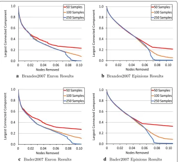
samples is less than 3 h. Again, it is interesting to compare to Bader2007. Accuracy results for both algorithms are visualized in Fig. 4. Note that concerning accuracy, both algorithms are almost identical. With the Enron test, both algorithms achieve a cluster of less than 1% with removal of about 8.5% of vertices. With the Epinions dataset, both leave a largest cluster of less than 1% with the removal of approximately 7% of vertices. Note that speed-wise Brandes2007 takes roughly twice as long as Bader2007, using the same numbers of samples.
Bader et al. 2007 (Bader2007)
Like Brandes2007, this algorithm estimates centrality by solving the SSSP problem on a sampled subset of vertices. The sampling is referred to as adaptive, because the number of samples required can vary depending on the information obtained from each sample [19]. As with other sampling algorithms, the speedup achieved is directly proportional to the number of shortest path computations. In the worst case, all vertices would be sampled, and so the time complexity of this algorithm is O(|V||E|) in the worst case, and O(k|E|), where k is the number of samples, in the practical case. There are two parameters to this algorithm. The first is a constant c that controls a stopping condition. The second parameter is an arbitrary vertex. For optimum performance, the arbitrary vertex should have high betweenness centrality.
0.0 0.2 0.4 0.6 0.8 1.0 tn en op mo C de tc en no C t se gr aL Nodes Removed 50 Samples 100 Samples 250 Samples
0 0.02 0.04 0.06 0.08 0.10
a Brandes2007 Enron Results
0.0 0.2 0.4 0.6 0.8 1.0 tn en op mo C de tc en no C t se gr aL Nodes Removed 50 Samples 100 Samples 250 Samples
0 0.02 0.04 0.06 0.08 0.10
b Brandes2007 Epinions Results
0.0 0.2 0.4 0.6 0.8 1.0 tn en op mo C de tc en no C t se gr aL Nodes Removed 50 Samples 100 Samples 250 Samples
0 0.02 0.04 0.06 0.08 0.10
c Bader2007 Enron Results
0.0 0.2 0.4 0.6 0.8 1.0 tn en op mo C de tc en no C t se gr aL Nodes Removed 50 Samples 100 Samples 250 Samples
0 0.02 0.04 0.06 0.08 0.10
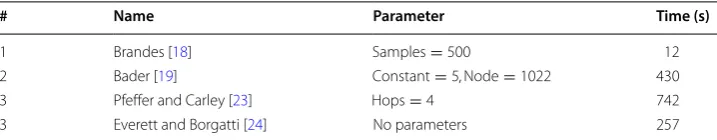
The algorithm is of great interest because its benchmark time was the fastest in [17], where the algorithm is referred to as GSIZE. We used code from [17] to run tests of four approximation methods, calculating betweenness centrality values for the Enron dataset. Results from this experiment are shown in Table 6.
It seems very clear that the fastest method here is Brandes2007, and yet results presented in [17] show that the Bader method is overall ten times faster than the others. Interestingly, by experimenting with the arbitrary vertex parameter, we were able to obtain a range of execution times from 430 to 3 s, depending on the choice of vertex. Obviously, this makes benchmarking the speed of the algorithm difficult.
The benchmarking method in [17] only calculates once on the initial graph. There-fore, it is easy to pick one high-betweenness vertex, perhaps by guessing based on degree. The clustering and immunization tests in this work calculate betweenness centralities repeatedly on a changing graph. There is no way to know what the high-est betweenness vertices are at a given time. One easy-to-calculate proxy is ver-tex degree. Running the algorithm with a parameter of c=2 , and pivoting on the
highest degree vertex at each step, our 10,000-node Graph 1 was clustered at 100% accuracy in 8960 s. Compare this to 290 s for Brandes2007. A second attempt was made to speed the algorithm up by, at each iteration, choosing the second highest betweenness centrality vertex from the previous iteration. This also did not speed things up. Bader et al. state in [19] that they set a limit on the number of samples at n
20 . We tried this and noticed that with Graph 1 the stopping condition was never reached—500 samples were always used. This configuration clustered perfectly again, but was still not fast at 1112 s. Last, we tried simply changing the limits on the number of samples. With limits of 50, 100 and 250 we got acceptable speeds and accuracies. All tests were run with parameter c=2 , although the parameter
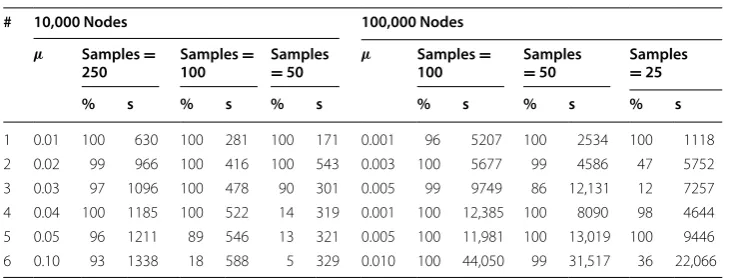
prob-ably was not used as the number of samples in fact controlled the stopping point. Results for the clustering test are shown in Table 7. With a small number of 50 samples, this algorithm clustered the 10,000-node graph 1 in 171 s with 100% accu-racy. Clustering the most difficult graph, the 100,000-node Graph 6, to over 90% accuracy took 8.75 h. It is noted on the immunization tests that the 50 sample test was largely ineffective, while the 250 sample test was much more successful, with the largest remaining cluster of only 1.1% with approximately 9% of vertices removed. These results can be seen in Table 8. Accuracy results for the immunization test are compared with Brandes2007 in Fig. 4.
Table 6 Initial testing of four algorithms on the Enron dataset
# Name Parameter Time (s)
1 Brandes [18] Samples=500 12
2 Bader [19] Constant=5 , Node=1022 430
3 Pfeffer and Carley [23] Hops=4 742
Geisberger et al. better approximation (Geisberger2008)
This algorithm is developed by Geisberger et al. [21]. It is based on the pivot method originally proposed by Brandes and Pich, where calculations are run on some number k of sampled pivots. The Brandes2007 method is said to overstate the importance of nodes near a pivot, a problem that this method solves by using a linear scaling func-tion to reestimate betweenness centrality values based on the distance a from a node to a pivot. Overall time complexity of the method is O(|V||E|), where the speedup is proportional to the number of pivots, k, that are sampled. What will perhaps turn out to be the true power of this algorithm is realized by the authors’ statement that the “algorithms discussed are easy to parallelize with up to k processors” [21]. We used the implementation in NetworKit [74], in the version which parallelizes the compu-tations. The parallelization is programmed using Open MPI. The only parameter is the number of samples, which is chosen by the user. In [21] the number of samples is chosen as powers of 2, ranging from 16 to 8192. We had surprisingly good luck with sample sizes as small as 2. Results for the clustering test are shown in Table 9. This is a quick method to use for clustering with high accuracies on both the 10,000 and 100,000 graphs. Note especially the performance on the most difficult graphs. This is an algorithm that scales to a difficult graph with a large number of edges much better than those we have seen so far. See Figs. 1 and 2 for a comparison of Geisberger2008 performance among the fastest of the algorithms tested.
Results from the immunization test are listed in Table 10. It is interesting to note that, while the improvement from 4 samples to 8 is large for both Enron and Epinions, the improvement from 8 to 16 samples is not as large. Overall, this is a highly accurate algorithm. This is especially evident in Fig. 5.
Table 7 Bader2007 clustering results for LFR nets of 10,000 and 100,000 nodes
# 10,000 Nodes 100,000 Nodes
µ Samples =
250 100Samples = Samples = 50 µ 100Samples = Samples = 50 Samples = 25
% s % s % s % s % s % s
1 0.01 100 630 100 281 100 171 0.001 96 5207 100 2534 100 1118 2 0.02 99 966 100 416 100 543 0.003 100 5677 99 4586 47 5752 3 0.03 97 1096 100 478 90 301 0.005 99 9749 86 12,131 12 7257 4 0.04 100 1185 100 522 14 319 0.001 100 12,385 100 8090 98 4644 5 0.05 96 1211 89 546 13 321 0.005 100 11,981 100 13,019 100 9446 6 0.10 93 1338 18 588 5 329 0.010 100 44,050 99 31,517 36 22,066
Table 8 Bader2007 run time and max cluster size immunization results
Dataset Samples=50 Samples=100 Samples=250
Seconds Max size (%) Seconds Max size (%) Seconds Max size (%)
Enron 109 19.7 228 2.0 597 0.1
Gnutella 1074 47.2 2262 35.7 5721 14.0
Riondato–Kornaropoulos fast approximation through sampling (Riondato2016)
Riondato and Kornaropoulos introduce this method in [20], which is based on sampling a predetermined number of node pairs (chosen uniformly at random). The sample size is based on the vertex diameter of the graph, denoted VD(G), which is the minimum number of nodes in the longest shortest path in G, and may vary from (diameter + 1) if the graph is weighted. Sampled vertices can be chosen to guarantee that the estimated betweenness val-ues for all vertices are within an additive factor ǫ from the real values, with a chosen prob-ability at least 1-δ , where 0< δ <1.
The time complexity of this algorithm is O(r(|V| + |E|)) , where r is determined by the equation:
(3) r= c
ǫ2
⌊log2(VD(G)−2)⌋ +1+ln1
δ
.
Table 9 Geisberger2008 clustering results for LFR nets of 10,000 and 100,000 nodes
# 10,000 nodes 100,000 nodes
µ Samples
= 16 Samples = 8 Samples = 4 µ Samples = 8 Samples = 4 Samples = 2
% s % s % s % s % s % s
1 0.01 100 285 100 191 100 141 0.001 100 3694 100 3040 95 2002 2 0.02 99 415 100 256 98 187 0.003 100 3790 92 3129 100 2508 3 0.03 95 478 97 296 98 207 0.005 100 4339 100 3577 98 2680 4 0.04 98 519 98 314 100 217 0.001 97 8993 100 6934 96 6421 5 0.05 100 545 98 329 98 218 0.005 100 10,885 100 9180 95 7862 6 0.10 95 607 95 360 97 233 0.010 100 16,307 10 12,456 100 9844
Table 10 Geisberger2008 run time and max cluster size immunization results
Dataset Samples=4 Samples=8 Samples=16
Seconds Max size (%) Seconds Max size (%) Seconds Max size (%)
Enron 94 19.5 187 0.4 254 0.2
Gnutella 1360 <0.01 2063 <0.01 3414 <0.01
Epinions 1434 47.8 3491 0.2 5825 0.05
0.0 0.2 0.4 0.6 0.8 1.0 tn en op mo C de tc en no C t se gr aL Nodes Removed 4 samples 8 samples 16 samples
0 0.02 0.04 0.06 0.08 0.10
a Enron
0.0 0.2 0.4 0.6 0.8 1.0 tn en op mo C de tc en no C t se gr aL Nodes Removed 4 Samples 8 Samples 16 Samples
0 0.02 0.04 0.06 0.08 0.10
In Eq. 3, c is a universal positive constant that is estimated in [20] to be 0.5, VD(G) is the vertex diameter of the graph, ǫ is the additive factor by which the approximation may vary from the true betweenness centrality value, and δ is the probability that the esti-mated value will be within ǫ of the true value.
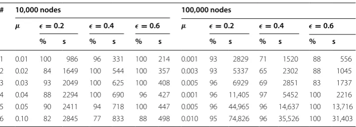
We used the implementation in NetworKit [74]. There are three parameters, the first of which, a constant c, is set at 1.0 in NetworKit. The other parameters are ǫ , which is the maximum additive error, and δ , which is the probability that the values are within the error guarantee. Our experiments use δ=0.1 for a probability of 90%, and vary ǫ , where higher ǫ values mean lower accuracy but also greater speed. Results are shown in Table 11. A couple of things are interesting. First, notice that relatively good accura-cies are obtained even at relatively high values of ǫ . The algorithm displays good speeds on the simpler 100,000-node graphs, taking only 556 s to cluster Graph 1 compared to 2808 s for Geisberger2008. However, Riondato2016 does not scale as well—the most dif-ficult graph takes about three times as long as Geisberger2008 to cluster with at least 90% accuracy.
Results from the immunization test are shown in Table 12 and Fig. 6.
Overall, Riondato2016 is the fourth most successful of our survey, and offers a theoret-ical guarantee of accuracy. A similar theorettheoret-ical guarantee is also offered by Borassi2016.
McLaughlin and Bader Hybrid‑BC (McLaughlin2014)
Hybrid-BC is introduced by McLaughlin and Bader in [41]. It offers an approxima-tion that uses a sampling of k vertices to determine the structure of the graph. As k is increased, calculations are slower, but accuracy is greater.
McLaughlin2014 is a GPU-based algorithm, and calculations were initially performed and timed on a computer with an Nvidia GeForce GTX 1080 GPU, which has 2560 Table 11 Riondato2016 clustering results for LFR nets of 10,000 and 100,000 nodes
# 10,000 nodes 100,000 nodes
µ ǫ=0.2 ǫ=0.4 ǫ=0.6 µ ǫ=0.2 ǫ=0.4 ǫ=0.6
% s % s % s % s % s % s
1 0.01 100 986 96 331 100 214 0.001 93 2829 71 1520 88 556 2 0.02 84 1649 100 544 100 357 0.003 93 5337 65 2302 88 1045 3 0.03 93 2049 100 625 100 408 0.005 96 6929 69 2851 83 1737 4 0.04 88 2294 100 690 96 427 0.001 96 11,405 97 5452 100 2216 5 0.05 90 2411 94 718 100 447 0.005 96 44,965 96 14,637 100 13,716 6 0.10 82 2845 77 833 88 498 0.010 95 74,826 96 35,526 100 31,403
Table 12 Riondato2016 run time and max cluster size immunization results
Dataset ǫ=0.6 ǫ=0.4 ǫ=0.2
Seconds Max size (%) Seconds Max size (%) Seconds Max size (%)
Enron 4346 25.0 7590 20.2 25,131 5.4
Gnutella 2550 10.0 4517 0.6 14,946 0.1
CUDA cores, 20 streaming multiprocessors, and a base clock of 1607MHz. This GPU is at this writing found in good-quality gaming computers, and is at a price point that most practitioners can afford. It is arguably Nvidia’s second or third most powerful GPU. We used code downloaded from Adam McLaughlin’s website [41]. Our hardware setup was capable of running 1024 threads simultaneously.
Results for the clustering test are shown in Table 13. Across the board, these are the best results we have seen so far. In fact, McLaughlin2014 is able to cluster the most diffi-cult graph with a high 98% accuracy in approximately 60% of the time of Geisberger2008. It is noted that McLaughlin2014 is one of the fastest and most accurate of all algorithms on the clustering test.
Results for the immunization test are shown in Table 14. The times are the fastest seen so far, and the the max cluster sizes are small. As can be seen in Fig. 7, 64 samples pro-duced the best result in all cases, but 32 samples also performed well. Notice the large difference in accuracy between those and the test with 16 samples. Also notice that due to somewhat lower accuracy on the Enron test, we have changed the scale of the x-axis. The McLaughlin algorithm is interesting because it scales very well time-wise, but accu-racies are not as good. It does better on the clustering test, but is also very successful on the immunization test.
0.0 0.2 0.4 0.6 0.8 1.0
tn
en
op
mo
C
de
tc
en
no
C t
se
gr
aL
Nodes Removed
e=0.6 e=0.4 e=0.2
0 0.02 0.04 0.06 0.08 0.10
a Enron
0.0 0.2 0.4 0.6 0.8 1.0
tn
en
op
mo
C
de
tc
en
no
C t
se
gr
aL
Nodes Removed
e=0.6 e=0.4 e=0.2
0 0.02 0.04 0.06 0.08 0.10
b Epinions Fig. 6 Visualization of results for Riondato2016 Immunization Test
Table 13 McLaughlin2014 clustering results for LFR nets of 10,000 and 100,000 nodes With Nvidia GTX1080 GPU
# 10,000 nodes 100,000 nodes
µ k=128 k=64 k=32 µ k=64 k=32 k=16
% s % s % s % s % s % s
The McLaughlin2014 results are so impressive that we wanted to determine the extent to which the properties of the GPU influenced calculation times. We replaced the Nvidia GeForce GTX 1080 GPU with an Nvidia Titan V GPU, which has 5120 CUDA cores (twice as many as the GTX1080), 80 streaming multiprocessors (four times as many as the GTX1080), and a base clock of 1200 MHz (interestingly, slower than the GTX1080). Results from rerunning the clustering test with this new con-figuration are shown in Table 15. For the 10,000-node graphs, clustering times are reduced by about 70%. The time to process 100,000-node Graph 6 with k = 64 went from 10917 to 6007 s, a savings of almost 82 min off an already fast 3-h processing time. These are among the best times that we will see.
Table 14 McLaughlin2014 run time and max cluster size immunization results
Dataset Samples=16 Samples=32 Samples=64
Seconds Max size (%) Seconds Max size (%) Seconds Max size (%)
Enron 60 7.6 110 0.1 121 0.1
Gnutella 219 51.1 332 41.6 597 16.8
Epinions 552 33.0 784 15.8 1087 6.5
0.0 0.2 0.4 0.6 0.8 1.0
tn
en
op
mo
C
de
tc
en
no
C t
se
gr
aL
Nodes Removed
16 Samples 32 Samples 64 Samples
0 0.04 0.08 0.12 0.16
a Enron
0.0 0.2 0.4 0.6 0.8 1.0
tn
en
op
mo
C
de
tc
en
no
C t
se
gr
aL
Nodes Removed
16 Samples 32 Samples 64 Samples
0 0.02 0.04 0.06 0.08 0.10
b Epinions Fig. 7 Visualization of results for McLaughlin2014 immunization test
Table 15 McLaughlin2014 clustering results for LFR nets of 10,000 and 100,000 nodes with Nvidia Titan V GPU
# 10,000 nodes 100,000 nodes
µ k=128 k=64 k=32 µ k=64 k=32 k=16
% s % s % s % s % s % s
1 0.01 95 88 100 69 100 68 0.001 100 2074 100 1831 99 1535
2 0.02 98 87 98 69 98 68 0.003 97 2084 97 1979 87 1678
3 0.03 100 88 100 69 100 67 0.005 93 2374 72 2224 14 1671 4 0.04 100 80 100 70 100 68 0.001 100 4613 100 4124 100 3629 5 0.05 98 79 94 69 100 67 0.005 100 4778 100 4385 100 3813
The performance of McLaughlin2014 on the clustering tests with the Titan V GPU is compared to the other top algorithms in Figs. 1 and 2. A comparison of immunization test results using the large Google graph is shown in Fig. 3. Interestingly, although it is still a top performer, it is sometimes bested by other algorithms in terms of speed and accuracy. At the time of this writing, the price of the Titan V was approximately five times the cost of the GTX 1080.
Borassi and Natale KADABRA (Borassi2016)
ADaptive Algorithm for Betweenness via Random Approximation (KADABRA) is described by Borassi and Natale in [30]. These authors achieve speed in two different ways. First, distances are computed using balanced bidirectional breadth-first search, in which a BFS is performed “from each of the two endpoints s and t, in such a way that the two BFSs are likely to explore about the same number of edges, and ... stop as soon as the two BFSs touch each other.” This reduces the time complexity of the part of the algo-rithm that samples shortest paths from O(|E|) to O(|E|12+o(1)) . A second improvement is that they take a different approach to sampling, one that “decreases the total number of shortest paths that need to be sampled to compute all betweenness centralities with a given absolute error.” The algorithm has a theoretical guarantee of error less than ǫ with probability 1 − δ . For our experiments, we kept δ at 0.1, which implied a 90% probability of being within the specified error, and varied ǫ.
Experiments with Borassi2016 were run using the original code as referenced in [30]. Results are shown in Table 16. Borassi2016 code is parallelized using OpenMP. Note that it is very fast, and that the accuracies are impressive, even at what seem to be high error tolerances. For example, the threshold time for the easiest 10,000-node graph is 60 s with no special hardware, where the same graph is clustered using an expensive GPU in 68 s. Notice that with the 100,000-node graphs, the ǫ=0.05 results from Borassi2016 are comparable with, and sometimes faster than, the k = 32 results from McLaughlin2014 with the Titan V GPU. The only issue we notice with the Borassi2106 algorithm is that the time seems to be very sensitive to small changes in ǫ . For example, our attempts to run the 100,000-node graphs at ǫ =0.01 were going to take hours longer than at ǫ=0.025 . Clustering 100,000-node Graph 6 with
ǫ=0.025 takes over twice as long as with the high-powered GPU, raising questions Table 16 Borassi2016 KADABRA clustering results for LFR nets of 10,000 and 100,000 nodes
# 10,000 nodes 100,000 nodes
µ ǫ=0.01 ǫ=0.05 ǫ=0.1 µ ǫ=0.025 ǫ=0.05 ǫ=0.1
% s % s % s % s % s % s
1 0.01 100 364 97 89 95 60 0.001 93 2378 95 578 72 417
2 0.02 99 335 97 94 98 68 0.003 97 2335 82 997 74 334
3 0.03 96 313 88 90 84 77 0.005 87 2955 88 1242 69 706
4 0.04 99 271 91 96 80 86 0.001 95 8288 95 2775 94 1227
about scalability; however, it appears that if one is willing to trade a small amount of accuracy, the speed of Borassi2016 rivals that of a GPU algorithm.
Results from the immunization test are shown in Table 17. Notice the extremely small largest components for all three networks when ǫ=0.01 , and the small sizes when ǫ=0.05 . Times are shorter than for any algorithms but McLaughlin2014. Accuracy results for the immunization test are shown in Fig. 8. Notice particularly in Fig. 8b the rapid decrease in size of the largest component with only 6% of nodes removed, and results for ǫ =0.05 and ǫ =0.01 are very similar. These results are so impressive that we ran the algorithm on the 875k-node Google graph. It achieved these accuracies: ǫ=0.1 : 53,706 s and 27.9% accuracy, ǫ=0.05 : 58,405 s and 11.7% accuracy, and ǫ =0.025 : 85,277 s and 8.7% accuracy. A comparison of Borassi2016 with the other two algorithms tested on the Google graph is shown in Fig. 3a. Notice that this is arguably the most successful of the three algorithms in terms of speed and accuracy. In Fig. 3b it shows by far the most rapid decline in largest component size, decreasing to less than 1% of graph size with less than 2% of nodes removed.
The Borassi2016 algorithm can be configured to return the top k vertices. In previous experiments we used it to return only the top vertex. Because the exact order of verti-ces chosen is not of the utmost importance in the clustering test, we wondered if the speed of this algorithm could be improved even further by choosing a set of nodes at each iteration. We tested this on the 10,000-node graphs by using the algorithm to find the top five vertices, while all other factors remained the same. Results can be seen in Table 18. The 10,000-node baseline graph is clustered in 36 s, compared to 68 s for the Table 17 Borassi2016 run time and max cluster size immunization results
Dataset ǫ=0.1 ǫ=0.05 ǫ=0.01
Seconds Max size (%) Seconds Max size (%) Seconds (%) Max size (%)
Enron 61 36.5 80 15.9 126 3.2
Gnutella 627 16.2 707 2.1 1867 1.0
Epinions 476 59.3 1093 8.5 2197 2.6
0.0 0.2 0.4 0.6 0.8 1.0
tn
en
op
mo
C
de
tc
en
no
Ct
se
gr
aL
Nodes Removed
e=0.1 e=0.05 e=0.01
0 0.02 0.04 0.06 0.08 0.10
a Enron
0.0 0.2 0.4 0.6 0.8 1.0
tn
en
op
mo
C
de
tc
en
no
Ct
se
gr
aL
Nodes Removed
e=0.1 e=0.05 e=0.01
0 0.02 0.04 0.06 0.08 0.10
GPU algorithm. The most difficult graph took 4402 s, which is 27 min shorter than the clustering time with the GPU.
Charts showing the overall performance of Borassi2016 compared to the other three top algorithms are contained in Figs. 1 and 2. Figure 2a is particularly interesting, as Borassi2016 beats all other algorithms with its combination of speed and accuracy.
Yoshida’s adaptive betweenness centrality (Yoshida2014)
Yoshida2014 adaptive betweenness centrality refers to computing betweenness central-ity for a succession of vertices “without considering the shortest paths that have been taken into account by already-chosen vertices” [1]. This description matches exactly the Greedy-BC heuristic used with NBR-Clust. Once the array of betweenness centralities is calculated, the node-removal order is known and the resilience measures are calculated for the graph at each configuration. The configuration with the lowest resilience meas-ure value is chosen. Yoshida’s adaptive betweenness centrality algorithm has an expected total runtime of O((|V| + |E|)k+hk+hk log |V|), where h is a probabilistic parameter that in most graphs is much less than (|V| + |E|) , and k is the number of times the graph is sampled. The algorithm runs faster or slower depending on the parameter k, which also controls the expected error. It is suggested that k should be chosen to be O(log |V|/ǫ2) , where ǫ is the expected error. Our experiments used different values of k to help establish a link between the speed and accuracy of this algorithm.
We used the original code downloaded from Yoshida’s website. Results for the cluster-ing test are shown in Table 19. We had success with this algorithm in [25], but here were unable to cluster the 100,000-node Graph 6 with 90% accuracy, even with k=800, 000 . Also, the corresponding times were comparatively long, and we did not continue with the immunization test.
Sariyüce et al. BADIOS (Sariyüce2012)
BADIOS (Bridges, Articulation, Degree-1, and Identical vertices, Ordering, and Side vertices) is introduced by Sariyüce et al. [32]. BADIOS is not actually an approxima-tion technique, but a speed enhancement. This algorithm involves splitting a graph in ways that will not affect the accuracy of the betweenness centrality calculation. Because the pieces are smaller, scaling problems are reduced. For example, Degree-1 means that all degree-1 vertices have a betweenness centrality of zero. They can be Table 18 Borassi2016 KADABRA clustering results for LFR nets of 10,000 and 100,000 nodes with top five vertices chosen
# 10,000 nodes 100,000 nodes
µ ǫ=0.01 ǫ=0.05 ǫ=0.1 µ ǫ=0.025 ǫ=0.05 ǫ=0.1
% s % s % s % s % s % s
1 0.01 100 115 100 44 98 36 0.001 94 1059 93 311 77 177
2 0.02 95 98 89 45 99 45 0.003 92 1270 96 477 76 283
3 0.03 91 95 85 47 98 46 0.005 95 1207 90 595 75 385
4 0.04 95 86 87 46 82 47 0.001 100 2898 98 1239 84 339
5 0.05 91 83 90 48 55 47 0.005 100 3216 94 1711 88 974
removed from a graph, shrinking its size without affecting the accuracy of the final calculation. It sounds simple, but even after a graph is shattered by removing an articulation node, that node becomes a degree-1 node and can be removed. The dif-ferent strategies are repeated until all options are exhausted.
In the worst case, manipulations to the graph fail or are few (for example, a graph with many large cliques), which indicates a time complexity of O(|V||E|). In the best case times are greatly enhanced. Our 10,000-node Graph 1 took approximately 5 h with BADIOS. This is a substantial improvement over the original exact calculation time of 48 h; however, the savings in time does not compare to the other approxima-tion algorithms discussed.
Sariyüce et al. gpuBC (Sariyüce2013)
Sariyüce et al. introduced gpuBC in 2013. It contains some ideas from BADIOS, such as removal of degree 1 vertices and graph ordering. It also introduces new ideas: first, vertex virtualization, which replaces high-degree vertices with virtual vertices that have at most a predetermined maximum degree. One of the original problems with GPU parallelization of betweenness centrality is whether to parallelize based on edge or node traversals. By evening out the degree of vertices, this method solves the problem. Second, they use techniques to store the graph that improve the speed of memory access.
The software is available on their website. The software is written for CUDA 4.2.9. We could not get it to run with more recent versions (at this writing, CUDA 9.1 is the most recent version). We were able to run gpuBC for the 10,000-node graphs after installing older versions of Linux and CUDA. Due to memory errors that we could not correct, we were not able to run gpuBC on the 100,000-node graphs.
We used the version of the software with ordering and degree-1 vertex removal techniques enabled, and virtual-vertex based GPU parallelism with strided access. There are two parameters available, one is the max degree of the virtual vertex, which we set at 4, and the number of BFS runs to be executed, which we varied from 100 to 200 to 1000. Results for the clustering test are shown in Table 20, and they are good, although we could not get the Graph 6 to cluster to 90% accuracy.
Table 19 Yoshida2014 clustering results for LFR nets of 10,000 and 100,000 nodes
# 10,000 nodes 100,000 nodes
µ k=640, 000 k=160, 000 k=20, 000 µ k=800, 000 k=200, 000 k=60, 000
% s % s % s % s % s % s