www.adv-radio-sci.net/11/31/2013/ doi:10.5194/ars-11-31-2013
© Author(s) 2013. CC Attribution 3.0 License.
Radio Science
Electromagnetic diffraction and scattering of a complex-source
beam by a semi-infinite circular cone
H. Br ¨uns and L. Klinkenbusch
Institut f¨ur Elektrotechnik und Informationstechnik, Christian-Albrechts-Universit¨at zu Kiel, Germany
Correspondence to: L. Klinkenbusch ([email protected])
Abstract. A complex-source beam (CSB) is used to inves-tigate the electromagnetic scattering and diffraction by the tip of a perfectly conducting semi-infinite circular cone. The boundary value problem is defined by assigning a complex-valued source coordinate in the spherical-multipole expan-sion of the field due to a Hertzian dipole in the presence of the PEC circular cone. Since the incident CSB field can be interpreted as a localized plane wave illuminating the tip, the classical exact tip scattering problem can be analysed by an eigenfunction expansion without having the conver-gence problems in case of a full plane wave incident field. The numerical evaluation includes corresponding near- and far-fields.
1 Introduction
Scattering and diffraction of a plane electromagnetic wave by a semi-infinite perfectly electrically conducting (PEC) cir-cular cone has often been treated in the literature. A survey on this subject can be found in the classical monograph by (Bowman et al., 1987). More recently, the scattered field has been obtained by a multipole-based integration of the ex-act surface-currents for the case of an incident plane wave. However, that solution suffers from a missing convergence of the finally obtained multipole series, and the application of suitable series-transformation techniques has been necessary to asymptotically derive the corresponding limiting values (Klinkenbusch, 2007; Kijowski and Klinkenbusch, 2011). Particularly, we are interested in the fields related the cone’s apex, as the corresponding scattered field can act as a further element to complete asymptotic methods like the Geometri-cal Theory of Diffraction (GTD) and the Uniform Theory of Diffraction (UTD).
For the analysis of the influence of the tip on the scat-tered field, we have used a localized plane wave, that is, a
complex-source beam (CSB) as the incident field. This can be achieved by simply assigning a complex-valued location to a dipole source. The width, focus length, and direction of incidence of the CSB can be controlled nearly arbitrar-ily (Orlov and Peschel, 2010). Combining this powerful tool with the spherical-multipole expansion provides a conver-gent eigenfunction solution with focusses on the evaluation of the scattered related to the tip of the cone.
Section 2 summarizes the solution of Maxwell’s equations in the presence of a PEC circular cone, and in Sect. 3 the complex-source technique is introduced. Finally, we present some numerical results in Sect. 4.
2 Solution of Maxwell’s equations in the presence of a PEC semi-infinite circular cone
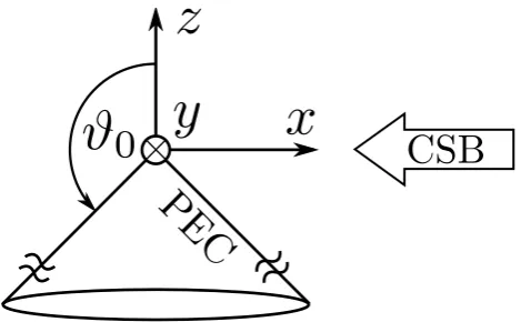
Consider a perfectly electrically conducting (PEC) circular cone as illustrated in Fig. 1 with a half outer opening angle ϑ0 embedded in a homogeneous medium with permittivity εand permeability µ. We are looking for a solution of the time-harmonic Maxwell’s equations at a time factore+j ωt. 2.1 Helmholtz equation in spherical coordinates
The homogenous scalar Helmholtz equation
18(r, ϑ, ϕ)+κ28(r, ϑ, ϕ)=0 (1)
with the wave numberκ=ω√εµcan be solved in spherical coordinatesr, ϑ, ϕ (ϑ represents the polar coordinate.) by a classical separation ansatz. We finally obtain the following elementary solution
Fig. 1. A PEC, semiinfinite, circular cone located on the negative z-axis. The half outer opening angle isϑ0. A CSB incides fromx -direction.
withzνbeing spherical Bessel functions related to (ordinary)
Bessel functions by zν(κr)=
r π
2κrZν+1/2(κr) (3)
Particularly we will need (everywhere regular) spherical Bessel functions of the first kind,jν(κr), and spherical
Han-kel functions of the second kind,h(ν2)(κr), satisfying the
ra-diation condition at the chosen time factore+j ωt. The spherical harmonicsYνm(ϑ, ϕ)are defined as
Yνm(ϑ, ϕ)=NνmPνm(cosϑ )ej mϕ, (4) that is, as products of associated Legendre functions of the first kindPνm(cosϑ )inϑ, and harmonic functions inϕ. The normalization constantNνmis chosen such that
ϑ0 Z 0 2π Z 0
Yνm(ϑ, ϕ) 2
sinϑ dϑ dϕ=1. (5)
2.2 Determination of eigenvalues
For the given geometry the solution has to be 2π-periodic inϕ, hence the eigenvaluesmhave to be integral. In order to get solutions of the Helmholtz equation for a PEC circu-lar cone as depicted in Fig. 1, these solutions have to ful-fill the boundary conditions on the cone’s surface. Therefore we need spherical harmonics that satisfy the Dirichlet condi-tion as well as spherical harmonics that satisfy the Neumann condition atϑ=ϑ0. This can be achieved by finding eigen-valuesνd andνn(Blume and Krebs, 1994) according to the
transcendental equations Pνm
d(cos ϑ )|ϑ0 =0 (6)
∂Pνm
n(cos ϑ )
∂ϑ ϑ 0
=0 (7)
which have been solved by means of a suitable numerical procedure, e.g. a bisection method.
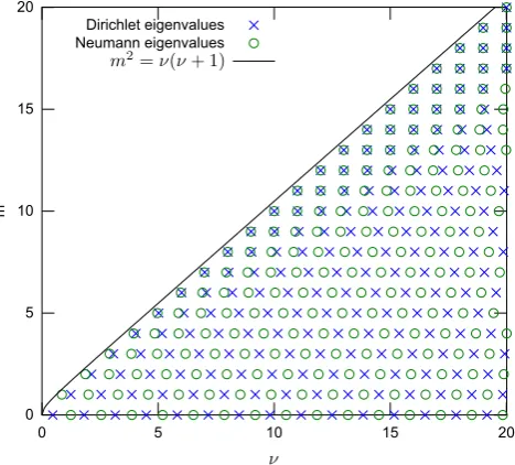
Moreover, it has been shown by (Katsav et al., 2012) that for all valid eigenvalue pairs (ν, m) it holds that
m2≤ν(ν+1) . (8)
Figure 2 shows the eigenvalue pairs for ϑ0=135◦ and νmax=40 in theν, m-plane.
2.3 Spherical-multipole expansion
Within a homogeneous domain, any solution of Maxwell’s equations outside the sources can be constructed by means of a complete set of spherical-multipole functions defined by
M(r)=(r×∇) 8(r) (9)
N(r)= 1
κ∇×(r×∇)
8(r) (10)
provided that 8 is a solution of the scalar homogeneous Helmholtz Eq. (1). They are determined according to
Mν,m(r, ϑ, ϕ)=zν(κr)mν,m(ϑ, ϕ) (11)
Nν,m(r, ϑ, ϕ)= − zν(κr)
κr ν(ν+1)Yν,m(ϑ, ϕ)er − 1
κr d
dr[rzν(κr)]nν,m(ϑ, ϕ)
(12)
wheremandndenote the transvere multipole functions: mν,m(ϑ, ϕ)= −
1 sinϑ
∂Yν,m(ϑ, ϕ)
∂ϕ eϑ
+∂Yν,m(ϑ, ϕ)
∂ϑ eϕ
(13)
nν,m(ϑ, ϕ)=
∂Yν,m(ϑ, ϕ)
∂ϑ eϑ
+ 1 sinϑ
∂Yν,m(ϑ, ϕ) ∂ϕ eϕ.
(14)
To accomplish that the tangential part of the electric field vanishes on the PEC cone’s surface, the spherical-multipole expansion of the total field reads
E(r)=X
νd,m
aνI I (I )
d,mN
I I (I ) νd,m(r)+
Z j
X
νn,m
bI I (I )ν
n,mM
I I (I )
νn,m(r) (15)
and for the magnetic field H(r)= j
Z X
νd,m
aνI I (I )
d,mM
I I (I ) νd,m(r)+
X
νn,m
bI I (I )ν
n,mN
I I (I )
νn,m(r). (16)
0 5 10 15 20
0 5 10 15 20
m
Dirichlet eigenvalues Neumann eigenvalues
Fig. 2. Pairs of eigenvalues forϑ0=135◦,νmax=20.
whereνd andνn are eigenvalues of the Dirichlet and
Neu-mann type, respectively.Z=√µ/εrepresents the intrinsic wave impedance of the homogeneous domain. The indices (I )and(I I )stand for the use of spherical Bessel functions jν or spherical Hankel functions of the second kindh(ν2)are
used according to Eq. (17) (see also Sect. 4). The multipole amplitudesaνd,mandbνd,mcan be determined for a Hertzian
dipole source atr0electrically polarized inc
eaccording to aνI I (I )
d,m = −κ
2 0Z0
(−1)m νd(νd+1)
NI (I I )ν
d,−m(r
0
)·ce, (18)
bI I (I )ν
n,m = −j κ
2 0
(−1)m νn(νn+1)
MI (I I )ν
n,−m(r
0
)·ce. (19)
The electric far-field is found from the asymptotic form of the spherical Hankel function of the second kind for large arguments as
E∞(r)=
e−j κr κr
" X
νd,m
−jνdaI I
νd,mnνd,m (20)
+Z j
X
νn,m
j(νn+1)bI I
νn,mmνn,m
# .
For the evaluation of the scattered field, we simply need to subtract the incident field from the total field where the in-cident field is computed by a similar approach using a free space spherical-multipole expansion.
3 Complex-source beam
The complex-source beam (CSB) offers the possibility to de-scribe a focussed beam analytically. If a complex valued lo-cation is assigned to a dipole source, a Gaussian beam is
gen-erated. The beam’s focus, width, and direction can be con-trolled arbitrarily by the chosen complex location. The com-plex location vector of the source has the form
r0c=r0r−jr0i, (21)
wherer0
r gives the actual position of the beam’s waist and r0
ithe direction of incidence. The absolute value ofr
0
i
corre-spond to the rayleigh length of the generated Gaussian beam. To clarify this, we insert a complex r0 into the free space Green’s function. We choose a purely imaginary locationr0:
r0= −j z0ez. (22)
That means, the beam has a rayleigh lengthz0, has it’s waist in the origin, and propagates inz-direction. Assuming a small distanceρ=px2+y2from the z-axis, a second order taylor series expansion of|r−r0|delivers a paraxial approximation:
|r−r0| = q
x2+y2+(z+j z
0)2 (23)
≈ (z+j z0)+ 1 2
ρ2 (z+j z0)
!
, ρz, z >0 Inserting Eq. (23) into the Green’s function we get: G(r,r0)= 1
4π
e−j κ|r−r0|
|r−r0| (24)
≈ 1
4π(z+j z0)
exp −j κ(z+j z0)− j κρ2 2(z+j z0)
!
= exp(κz0) 4π(z+j z0)
exp
−j κz− j κρ 2
2
z+z 2 0
z
−
ρ2
2z0
κ
1+z2
z02
.
Ignoring the factor exp(κz0)/4π(z+j z0), the result of Eq. (24) directly correspond to the form of the Gaussian beam:
exp(−j κz)exp −j κρ 2
2R(z) !
exp − ρ 2
w2(z) !
. (25)
By comparing Eqs. (24) and (25) we can identify following beam parameters: The radius of curvatureRis
R(z)=z+z 2 0
z . (26)
The radiuswof the beam is
w(z)=w0 s 1+ z z0 2 , (27)
wherew0is the radius at the waist: w0=
r 2z0
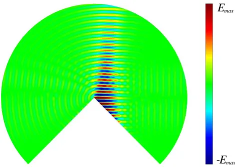
Fig. 3.Eyin thex, z-plane.
As we can see in Eq. (26), the radius of curvature gets large for zz0. That means that there are nearly plane wave fronts close to the beam’s waist which are – due to the trans-verse Gaussian profile – also localized.
4 Treatment of a complex-valued coordinate in the spherical-multipole expansion
The following equations are special cases of the Gegenbauer addition theorem applied to spherical Bessel functions of ze-roth order
sin(κR)
κR =
∞
X
n=0
(2n+1)jn(κr)jn(κr0)Pn(cosγ ), (29)
−cos(κR)
κR =
∞
X
n=0
(2n+1)jn(κr)yn(κr0)Pn(cosγ ). (30)
They are valid for arbitrary complexr, r0, γ , κand provided that
|re±j γ|<|r0| (31) and
R= q
r2+r02−2rr0cosγ . (32)
Having two position vectorsr(r, ϑ, ϕ) andr0(r0ϑ0, ϕ0), the
distance|r−r0|between this positions can be expressed by
Rif we choose
cosγ =cosϑcosϑ0+sinϑsinϑ0cos(ϕ−ϕ0) . (33) By combining Eqs. (29), (30) and the relation
Pn(cosγ )=
4π 2n+1
+n
X
m=−n
Ynm(ϑ, ϕ)Ynm∗(ϑ0, ϕ0) (34)
Fig. 4.Hxin thex, z-plane within a range ofr≤20m.
we can construct a spherical multipole expansion of the scalar free space Green’s function:
g(r,r0)= 1 4π
e−j κ|r−r0|
|r−r0| (35)
=
∞
X
n=0
+n
X
m=−n
jn(κr)h(n2)(κr
0
)Ynm(ϑ, ϕ)Ynm∗(ϑ0, ϕ0).
This expansion is valid for any complex locationr0, if the
condition Eq. (31) is fulfilled. If it is not,randr0can be per-muted due to the Green’s function symmetry. This paper only deals with CSBs that point directly to the tip of the cone, so there is only a complexr0-component (Katsav et al., 2012). In this caseγis real and the condition that has to be fulfilled is
|r|<|r0|. (36)
This must be considered for the multipole expansions in sec-tion 2.3, particulary for Eq. (17), if a complex-source beam is used.
5 Numerical results
The following results are for a circular cone with a half open-ing angle of 45◦(ϑ0=135◦) and are calculated with multi-pole expansions according to the preceding sections using a maximum orderνmax=40. The coordinates of the CSB arer0=(12+j48)m,ϑ0=90◦,ϕ0=0◦; this means that the
Fig. 5.Hzin thex, z-plane withinr≤20m.
Fig. 6. Current density distribution on the cone’s surface in the re-gionr≤40m. View fromz-direction. The beam incides from right-hand side.
of the beam. In the shadow region of the cone we can clearly see diffracted spherically shaped wavefronts. Figure 4 and 5 show the x- and the z-component of the magnetic field. While the incident part of the magnetic field is polarized in z-direction, the reflected part is polarized inx. In both fig-ures diffracted parts can be found. Figure 6 shows the cur-rent density distribution on the cone’s surface, which can be calculated with
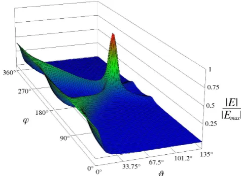
Js(r)= −eϑ×H(r)|ϑ=ϑ0. (37) There are two notable creeping waves in the shadow region of the cone. Finally, the magnitude of the scattered far-field is examined; in Fig. 7 it is shown in the form of a far-field pat-tern, in Fig. 8 it is plotted againstϑ, ϕ. The beam is reflected in every direction of ϕ; the highest values are observed in the direction of propagation. For 90◦< ϑ <135◦we observe two relatively small maxima, particulary in Fig. 8. This might
Fig. 7. Far-field pattern with the magnitude of the electric field.
Fig. 8. Magnitude of the electric far-field plotted againstϑ, ϕ.
be a consequence of the creeping waves, which can be ob-served in Fig. 6 of the current density.
6 Conclusions
The scattering of an electromagnetic CSB by a semi-infinite circular cone has been analysed using spherical multipole ex-pansions. Convergent results of the total or scattered field can be obtained for both near- and far-field. So far, only beams pointing directly to the tip of the cone have been considered. Future work will expand this approach to other geometries, e.g. elliptic cones. Furthermore the requirements for CSBs pointing in arbitrary directions will be investigated, so that other parts of the cone can be illuminated.
Acknowledgements. This work was supported by the Deutsche
References
Bowman, J. J., Senior, T. B. A., and Uslenghi, P. L. E., Electromag-netic and acoustic scattering by simple shapes (Revised Printing), Hemisphere Pub. Corp., New York, 1987.
Blume, S. and Krebs, V.: Der R¨uckstreuquerschnitt des semiin-finiten Kreiskegels, Arch. Elektrotech., 77, 239–244, 1994 Katsav, M., Heyman, E., and Klinkenbusch, L.: Complex-source
beam diffraction by an acoustically soft or hard circular cone, Electromagnetics in Advanced Applications (ICEAA), 2012 International Conference on, proceedings, Cape Town, South Africa, 2–7 September 2012, 135–138, 2012
Kijowski, M. and Klinkenbusch, L.: Eigenmode analysis of the electromagnetic field scattered by an elliptic cone, Adv. Radio Sci., 9, 31–71, 2011
Klinkenbusch, L.: Electromagnetic scattering by semi-infinite circular and elliptic cones, Radio Sci., 42, RS6S10, doi:10.1029/2007RS003649, 2007