R E S E A R C H L E T T E R
Open Access
Remarkable ground uplift and reverse fault
ruptures for the 2013 Bohol earthquake (Mw 7.1),
Philippines, revealed by SAR pixel offset analysis
Tomokazu Kobayashi
Abstract
By applying a pixel offset analysis using RADARSAT-2 SAR data to an inland crustal earthquake that occurred on Bohol Island, Philippines on 15 October 2013, we succeeded in mapping a ground displacement associated with the earthquake. The most concentrated crustal deformation with ground displacement exceeding 1 m is located in the northwest part of the island. The crustal deformation is zonally distributed and extends a length of approximately 50 km in the ENE–WSW direction. The ground in the mountainous area moved toward the satellite, while the ground in the northern coastal zone moved away from the satellite. A clear displacement discontinuity with a length of about 5 km, probably corresponding to earthquake surface faults, can be identified in the northeastern region. Our fault model consisting of two rectangular planes shows nearly pure reverse-fault motion on south-southeast-dipping planes with moderate dip angles. A local rupture occurs in the northeast at shallow depths and produces surface ruptures. By applying an additive color process using SAR amplitude images, significant changes in backscatter intensity were detected along the coast from Maribojoc to Loon; these changes suggest that the seafloor uplifted and the shoreline resultantly shifted seaward. The area showing the shoreline change is in good spatial agreement with the locally distributed large ground uplift predicted from our fault model. We identified a good correlation between the ground upheaval produced by the reverse-fault motion and elevation in the mountainous area, which is consistent with the idea that repeated historical reverse faulting developed the present-day topography.
Keywords:SAR; Pixel offset; Additive color process; Bohol earthquake; Crustal deformation; Earthquake surface fault; Shoreline changes; Fault model
Background
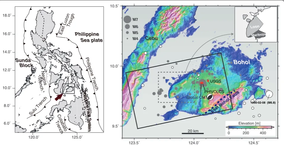
A devastating inland earthquake with moment magni-tude (Mw) of 7.1 struck Bohol Island, Philippines on 15 October 2013 [1]. Within the Philippine islands, which straddle a region of complex tectonics, Bohol Island is located in the Sunda block, beneath which the Philippine Sea plate subducts from the east westward. GPS data analyses and focal mechanism solutions suggest that the island is regionally subjected to E–W to NW–SE compression [2,3]. The Philippines have suffered from considerable historic seismic activity, mainly along the subduction zones and the Philippine fault zone (Figure 1), but the seismicity in and around Bohol Island has been
relatively low [4]. The largest previous earthquake that had occurred during the past several decades was the M6.8 event that occurred east of the island in 1990 (Figure 1), and no seismic events with a magnitude ex-ceeding 7 had occurred in the crust. The existence of the East Bohol fault in the southeast part of Bohol Island has been well known, however, the 2013 seismic event did not involve this fault but occurred along a previously undis-covered fault (hereafter called North Bohol fault).
One of the notable features of the seismic event was remarkable ground surface changes, which were ob-served in field surveys [5]. These changes included the appearance of earthquake surface faults with vertical off-sets of several meters and shoreline changes caused by
Correspondence:[email protected]
Geospatial Information Authority of Japan, Kitasato-1, Tsukuba, Ibaraki 305-0811, Japan
ground uplift. According to reports by the U. S. Geological Survey (USGS) and the Philippine Institute of Volcanology and Seismology (PHIVOLCS), among others, a reverse fault mechanism with a NW–SE compressive axis was in-ferred from seismic wave analyses, thus vertical ground movements associated with the reverse motion must have been involved in the ground surface changes. However, it remains unclear where and how the fault rupture contributed to these changes. Measurement of ground displacements around the epicentral area cer-tainly plays a key role in answering these questions, but there is no geodetic data from which we could obtain the detailed crustal deformation.
Satellite synthetic aperture radar (SAR) data can pro-vide detailed and spatially comprehensive ground infor-mation. Interferometric SAR (InSAR) analysis has the advantage of detecting ground deformation in a vast re-gion with high precision (e.g., [6,7]). However, for the Bohol event, the standard InSAR approach is not helpful for determining the details of the seismic rupture. Only C–or X-band SAR data are available for the event, thus it is not suitable to apply an InSAR method to measure ground displacement on Bohol Island, which is covered by forest [8-10]. We actually conducted an InSAR ana-lysis using the C-band data we handle in this study, but a coherent loss area resultantly spread over the island. Thus, in order to reveal the unknown surface displace-ments, we conducted a pixel offset method that enabled
us to robustly detect large ground deformation even in incoherent areas [11-13].
Methods
We used RADARSAT-2 data from the ascending orbit acquired on 12 January 2013 and 27 October 2013 for data analysis. This data pair provided the shortest tem-poral baseline among the SAR images covering the source region. The data obtained were strip-map im-agery (Wide Multi-Look Fine mode) with an incidence angle of 34.1° at the scene center. The area analyzed is indicated by the frame in Figure 1. We processed the SAR data from SLC products using a software package Gamma [14]. After conducting coregistration between two images acquired before and after the mainshock, we divided the single-look SAR amplitude images into patches and calculated the offset between corresponding patches by using an intensity tracking method. This method was performed by cross-correlating samples of backscatter intensity of a master image with those of a slave image [15]. A pixel offset is feasible even for such incoherent areas provided that a large correlation window is used to track similar speckle patterns [15]. We employed a nearly square search patch of 256 × 256 pixels (range × azimuth: ~680 m × ~640 m). We then reduced the artifact by applying an elevation-dependent correction incorporat-ing NASA Shuttle Radar Topography Mission (SRTM) digital elevation model (DEM) data with a 3-arcsec
˚ 5 . 4 2 1 ˚ 0 . 4 2 1 ˚ 5 . 3 2 1 9.5˚ 10.0˚ 10.5˚ 20 km M4 M5 M6 M7 Global CMT
0 200 400
Elevation [m]
PHIVOLCS USGS
1990-02-08 (M6.8) Bohol
Cebu
East Bohol Fault
6.0˚ 8.0˚ 10.0˚ 12.0˚ 14.0˚ 16.0˚ 18.0˚ P h ilipp ine F au ltS ys te m Philippine Sea plate Sunda Block
Sulu Trench TrenchCotabato
Philippine Trench East Luzon Trough
Negros Trench
120.0˚ 125.0˚
Maribojoc
Loon
resolution [16] in the same manner as used by Kobayashi et al. [13]. The measured offset consisted of two compo-nents: (1) displacement along the line of sight (range offset) and (2) horizontal movement along the ground parallel to the satellite track (azimuth offset).
Results and discussion
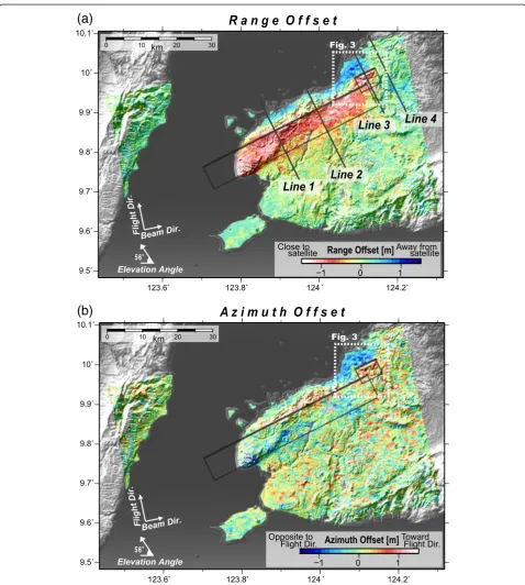
Ground displacement field for the 2013 Bohol earthquake Figure 2 shows the estimated range and azimuth offset fields over the entire analyzed area. The range offset analysis succeeded in mapping the ground displacement
(a)
(b)
in the proximity of the source region (Figure 2a). Inten-sive deformation was revealed in the northwest part of the island with ground displacement exceeding 1 m, and the deformation extends with a length of approximately 50 km in the ENE–WSW direction. The ground on the south side of the crustal deformation area (warm-col-ored area) moved toward the satellite, while the ground on the north side (cold-colored area) moved away from the satellite.
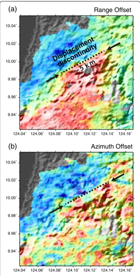
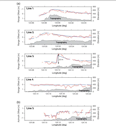
It is notable that a clear displacement discontinuity, across which the ground movement was in opposite direction, can be identified in the northeastern area (Figures 2a and 3a). Field surveys have discovered sur-face ruptures near the displacement boundary [5]. The length of the displacement boundary was estimated to be approximately 5 km, which is consistent with the field surveys. Figure 4 shows displacement profiles along the cross sections of lines 1–4 (shown in Figure 2). A sharp, large displacement offset suggesting a surface rup-ture can be seen in the line 3 profile. The observed offset is approximately 2 m, equivalent to a vertical movement of 2.4 m. The clearly identified displacement boundary terminates around the position of 124.13°E, 10.01°N, and large ground movement cannot be clearly seen farther northeast (line 4 in Figure 4a). On the other hand, except in the northeastern part, the displacement changes are relatively gradual (lines 1 and 2 in Figure 4a).
The azimuth offset field shown in Figure 2b is rather noisy. Crustal deformation produced by reverse-fault motion, in which northward/southward ground move-ment should be dominant, cannot be identified clearly. However, significant ground movement can be observed near the displacement discontinuity area with a relatively high signal-to-noise ratio. In this area, ground move-ment opposite to the satellite flight direction (cyan), i.e., nearly southward horizontal displacement, of approxi-mately 0.5 m can be recognized. The southward move-ment terminates at the displacemove-ment discontinuity observed in the range offset (Figure 3b).
Fault modeling
Based on the obtained displacement data, we tried to con-struct a fault model under the assumption of a rectangular fault with uniform slip in an elastic half-space [17]. A rect-angular fault model has the advantage that it can repre-sent a macroscopic feature of the source property with simple notation. A slip distribution model would have provided us with a more detailed picture regarding the fault rupture, but the result of the pixel offset analysis would not necessarily have enough measurement accuracy to estimate a more complex slip distribution. Thus, we here provide only a simple-shape fault model.
The offset field has ground surface changes over a vast range, and so produces too many values to be easily
assimilated in a modeling scheme. Thus, to reduce the number of data for the modeling analysis, we down-sampled the data beforehand, using a quadtree decom-position method. Essentially, we followed an algorithm presented by Jónsson et al. [18]. For a given quadrant, if, after removing the mean, the residue is greater than a prescribed threshold (25 cm in our case), the quadrant is further divided into four new quadrants. This process is iterated until either each block meets the specified cri-terion or the quadrant reaches a minimum block size
Displacement
discontinuity
(a)
(b)
Range Offset
Azimuth Offset
9.94˚ 9.96˚ 9.98˚ 10.00˚ 10.02˚ 10.04˚
124.04˚ 124.06˚ 124.08˚ 124.10˚ 124.12˚ 124.14˚ 124.16˚
9.94˚ 9.96˚ 9.98˚ 10.00˚ 10.02˚ 10.04˚
124.04˚ 124.06˚ 124.08˚ 124.10˚ 124.12˚ 124.14˚ 124.16˚
(8 × 8 pixels in our case). Upon application of the above-mentioned procedure, the size of the data set was reduced from 471070 to 405 for the range offset data. We also ap-plied the method in the same manner to the azimuth offset data. The azimuth offset data, however, were too noisy to incorporate into the modeling. Therefore, we used only
the data in the northeastern area, ranging from 124.00°E to 124.15°E and from 9.95°N to 10.10°N, where the signal-to-noise ratio was relatively high.
For the modeling, we applied a simulated annealing method for searching the optimal fault parameters [19,20]. We assumed a two-segment model that consists
0 200 400 600 800
Elevation [m]
−1
0
1
Range Offset [m]
Line 4
0 200 400 600 800
Elevation [m]
−1
0
1
Range Offset [m]
2.0 m
Line 3
Topography
Topography 0 200 400 600 800
Elevation [m]
−1
0
1
Range Offset [m]
Line 2
0 200 400 600 800
Elevation [m]
−1
0
1
Range Offset [m]
Line 1
(a)
(b)
0 200 400 600 800
Elevation [m]
1
0
Azimuth Offset [m]
−1
Longitude [deg]
Longitude [deg] Longitude [deg]
Longitude [deg]
Longitude [deg]
Topography Topography
Topography
Line 3
124.08 124.10 124.12 124.14 124.16
124.14 124.16 124.18 124.20 124.22
124.08 124.10 124.12 124.14 124.16
123.98 124.00 124.02 124.04 124.06
123.86 123.88 123.90 123.92 123.94
of a main fault producing the majority of the crustal de-formation and a local but essential fault located in the northeast producing clear surface offsets. For the main fault, we randomly assigned parameters within the search range of 123.75°–124.00° in longitude, 9.8°–9.9° in latitude, 0–20 km in depth, 0–70 km in length, 0– 30 km in width, 0°–90° (180°–270°) in strike, 0–90° in dip, 0°–180° in rake, and 0.0–10.0 m in slip amount. For the northeast fault, the clear displacement offsets reflect-ing surface ruptures strongly suggested that the fault rup-ture is rather shallow, thus we here fixed the fault top to be near the ground surface. With knowledge of the dis-placement discontinuity line, the search range of strike could be strongly limited to within 55°–65° (235°–245°) so as to fit the boundary line. We randomly assigned the other parameters within the search range of 124.10°– 124.15° in longitude, 9.85°–10.01° in latitude, 0–10 km in length, 0–30 km in width, 0–90° in dip, 0°–180° in rake, and 0–10.0 m in slip amount. To estimate the individual
confidence of each inferred parameter, we employed a bootstrap method [21].
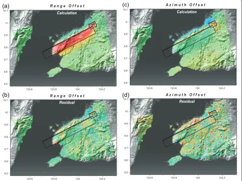
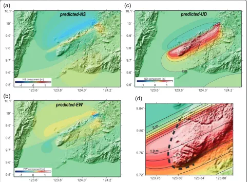
Figure 5 shows the range and azimuth offsets calcu-lated using our preferred model and the residuals be-tween the observations and calculations. The estimated fault parameters are listed in Table 1. Our model was able to reproduce well the observations (Figures 4 and 5). The root mean square of the residuals in range offset was esti-mated to be 19.1 cm, which is comparable to or less than the typical measurement accuracy of pixel-offset analysis [13]. Thus, our uniform slip model sufficiently accounts for the nature of the source. Figure 6 shows the three-component displacement calculated from the fault model. From the calculations, we can recognize the remarkable characteristic that vertical displacement, particularly upheaval, is predicted to be dominant for the seismic event. Our fault model shows (1) a south-southeast-dipping fault plane with a dip angle of ~60° for the main fault and ~40° for the northeastern fault, (2) ENE–
WSW oriented strikes, and (3) nearly pure reverse-fault motions. The total seismic moment is estimated to be 5.7 × 10¹⁹ N m (Mw 7.1) with a rigidity of 34 GPa. Ac-cording to the results of the USGS, the PHIVOLCS, and the Global Centroid Moment Tensor Project (GCMT pro-ject), the moment magnitude was estimated to be Mw 7.1 (5.6 × 10¹⁹N m), Mw 7.2, and Mw 7.1 (5.6 × 10¹⁹ N m), respectively [1,22,23]. Our result is in good agreement with these.
Shoreline changes revealed by SAR analysis
Significant ground upheaval was reported to have oc-curred in the coastal zone from the Maribojoc to Loon municipalities, and the shoreline shifted seaward by tens of meters ([5]; Toto B. personal communication). Exam-ining the range offset field, relatively large displacements of approximately 1.5 m can be observed in and around the area (Figure 2). The narrow shoreline changes, however, could hardly be extracted by the pixel offset analysis Table 1 Fault parameters of our preferred model for the 2013 Bohol event
Fault Longitude Latitude Depth Length Width Strike Dip Rake Slip Mw
1 123.926 (0.011) 9.841 (0.011) 7.3 (1.0) 51.3 (3.9) 12.5 (3.2) 63.1 (1.6) 56.8 (8.3) 86.0 (7.4) 2.5 (1.4) 7.1 2 124.124 (0.009) 9.983 (0.025) 2.0 6.4 (1.3) 6.0 (6.0) 64.0 (3.5) 41.1 (11.6) 117.5 (18.1) 2.0 (0.9) 6.2
GCMT 124.06 9.86 12.0 - - 38/237 44/48 76/103 - 7.1
Units for length, width, and depth are kilometers; those of dip, strike, and rake are degrees, and the unit of slip is the meter. We define the location of each fault as the center. Moment magnitude is calculated with the rigidity of 34 GPa. The parenthesized numbers are standard deviation (1σ). In the lowest row, the fault parameters are from the Global CMT solution.
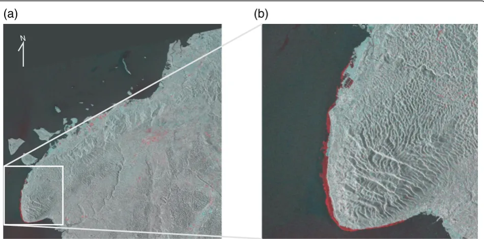
because of the low spatial resolution, thus detailed information about these could not be acquired. To overcome this difficulty, we attempted to obtain the ground surface changes by using the microwave back-scatter intensity of SAR amplitude images. For the ana-lysis, we basically followed an additive color process presented by Tobita et al. [24]. After coregisteration be-tween the two SAR images, we first assigned intensity variations in the pre-seismic amplitude image to varia-tions in cyan, (R, G, B) = (0%, 100%, 100%), and then vari-ations in the post-seismic image to red, (R, G, B) = (100%, 0%, 0%). Combining these two images, areas where backscatter increased / decreased / remained unchanged turned out to be red, cyan, and gray, respectively. Figure 7 shows the result of the additive color process. A clear red-colored zone can be observed extending in the coastal area from Maribojoc to Loon, where the backscatter in-tensity increased significantly. The total distance of the red zone is estimated to be about 13 km. We interpret it to mean that the seafloor uplifted and the shoreline shifted seaward resultantly.
The major source of error of this method is a tide-level difference between the two SAR data acquisition times. Thus, to confirm the validity of our analysis, we calculated it using Some Programs for Ocean-Tide Loading (SPOTL) software [25]. As a result, the differ-ence in tide level is approximately 9 cm in and around the sea area, thus there would be no serious affect in the analysis result.
Figure 6d shows the model-calculated vertical dis-placement in and around Maribojoc and Loon, where our fault model predicts a large ground uplift of approxi-mately 1.2 m (at maximum). Compared with other coastal areas, this area is locally subjected to large upheaval. A dotted line indicates the coastal zone showing the increase of backscatter intensity (Figure 7b). The locally distributed large uplift can account for the fact that shoreline changes occurred only in this area.
Relationship between ground movement and topography There is a good spatial correlation between the range shortening area (warm-colored area) and the mountain-ous area (Figure 2). In particular, the relationship is obvi-ous in the area from the coast to the north-facing slope of the mountain (lines 1 and 2 in Figure 4). The correl-ation between the two caused us to think about the landform evolution and whether the spatial correlation could be true. As mentioned in Section Methods, we applied an elevation-dependent correction to reduce the artifact displacement correlating with elevation, but the correction was often insufficient because of the large amount of topographic relief and the accuracy of the DEM data [13]. Thus, we had to consider carefully whether or not the spatial correlation is true. We here confirmed the potential error caused by the topography. For the SAR data pair that we analyzed, the perpendicular baseline of satellite orbit was estimated to be approximately−47 m at the scene center. In this case, the artifact, calculated
N
(a)
(b)
using a formulation presented by Kobayashi et al. [26], should be at most 8 cm at the elevation of 500 m. Thus, we concluded that the error produced by the topo-graphic effect can be ignored in this analysis.
Figure 8b shows the range offsets as a function of elevation for the analyzed domain indicated by the frame in Figure 8a. There is a good correlation be-tween the range offsets that consist mainly of vertical movement and the elevation, with a correlation coeffi-cient of 0.71. We may thus state that the reverse fault motion is in quite good harmony with the orientation of the long-term cumulative displacement in that the mountainous area is on the side of the hanging wall producing ground uplift. This may support the idea that reverse-fault motions have occurred repeatedly on
the North Bohol fault and may have contributed to the development of the present-day topography, although there is no clear evidence on the ground surface indicat-ing it to be an active fault.
Conclusions
We applied a pixel offset method using RADARSAT-2 SAR data to the 2013 Bohol earthquake and succeeded in mapping the crustal deformation. The following con-clusions were derived from the analyses.
(1) Intensive deformation with ground displacement exceeding 1 m extends in the northwest part of the island.
(2) The crustal deformation zone has a length of approximately 50 km in the ENE–WSW direction. (3) The ground on the southern side of the crustal
deformation area moved toward the satellite, while the ground on the northern side moved away from the satellite.
(4) A clear displacement discontinuity with a length of about 5 km, probably corresponding to earthquake surface faults observed in field surveys, can be identified in the northeastern part of the source region.
(5) Our fault model shows nearly pure reverse-fault motions on south-southeast-dipping planes with moderate dip angle. In the northeast, a local fault rupture occurs at shallow depths, causing the appearance of surface ruptures.
(6) Remarkable changes in backscatter intensity were detected along the coast from Maribojoc to Loon by applying an additive color process, and these changes suggest that the seafloor uplifted and the shoreline resultantly shifted seaward.
(7) The ground displacements produced by the reverse-fault motion are correlated with elevation, possibly suggesting that reverse-fault motions on the North Bohol fault have repeated historically and have contributed to the development of the present-day topography.
Competing interests
The author declares that he has no competing interests.
Acknowledgments
We used Generic Mapping Tools (GMT) provided by Wessel and Smith [27] to construct the figures. We are grateful to Dr. Toto, staff member at PHIVOLCS, for providing valuable information on the 2013 Bohol earthquake. We thank two anonymous reviewers and the editor (Prof. Satake) for their helpful comments to improve our manuscript.
Received: 5 December 2013 Accepted: 17 February 2014 Published: 14 April 2014
References
1. US Geological Survey (2013) M7.1 - 5km SE of Sagbayan, Philippines (BETA). http://comcat.cr.usgs.gov/earthquakes/eventpage/usb000kdb4#summary. Accessed 18 Nov 2013
2. Rangin C, Pichon XL, Mazzotti S, Pubellier M, Chamot-Rooke N, Aurelio M, Walpersdorf A, Quebral R (1999) Plate convergence measured by GPS across the Sundaland/Philippine Sea Plate deformed boundary: the Philippines and eastern Indonesia. Geophys J Int 139:296–316
3. Kreemer C, Holt WE, Goes S, Govers R (2000) Active deformation in eastern Indonesia and the Philippines from GPS and seismicity data. J Geophys Res 105:663–680
4. Acharya HK, Aggarwal YP (1980) Seismicity and tectonics of the Philippine Islands. J Geophys Res 85:3239–3250
5. Philippine Institute of Volcanology and Seismology (2013) QRT Report of investigation conducted on 16–25 October 2013. http://www.phivolcs.dost. gov.ph. Accessed 18 Nov 2013
6. Massonnet D, Feigl KL (1998) Radar interferometry and its application to changes in the earth’s surface. Rev Geophys 36:441–500
7. Bürgmann RP, Rosen A, Fielding EJ (2000) Synthetic aperture radar interferometry to measure Earth’s surface topography and its deformation. Annu Rev Earth Planet Sci 28:169–209
8. Zebker HA, Villasenor J (1992) Decorrelation in interferometric radar echoes. IEEE Trans Geosci Remote Sens 30:950–959
9. Rosen PA, Hensley S, Zebker HA, Webb FH, Fielding EJ (1996) Surface deformation and coherence measurements of Kilauea Volcano, Hawaii, from SIR-C radar interferometry. J Geophys Res 101:23109–23125
10. Wei M, Sandwell DT (2010) Decorrelation of L-band and C-band interferometry over vegetated areas in California. IEEE Trans. Geosci Remote Sens 48:2942–2952
11. Michel R, Avouac JP, Taboury J (1999) Measuring ground displacements from SAR amplitude images: application to the Landers earthquake. Geophys Res Lett 26:875–878
12. Tobita M, Murakami M, Nakagawa H, Yarai H, Fujiwara S, Rosen PA (2001) 3-D surface deformation of the 2000 Usu eruption measured by matching of SAR images. Geophys Res Lett 28:4291–4294
13. Kobayashi T, Takada Y, Furuya M, Murakami M (2009) Locations and types of ruptures involved in the 2008 Sichuan Earthquake inferred from SAR image matching. Geophys Res Lett 36. doi:10.1029/2008GL036907
14. Wegmüller U, Werner CL (1997) Gamma SAR processor and interferometry software. In: Proceedings of the 3rd ERS Symposium, vol SP-414. ESA, Florence, pp 1686–1692
15. Strozzi T, Luckman A, Murray T, Wegmuller U, Werner CL (2002) Glacier motion estimation using SAR offset-tracking procedures. IEEE Trans Geosci Remote Sens 40:2384–2391
16. Farr TG, Rosen PA, Caro E, Crippen R, Duren R, Hensley S, Kobrick M, Paller M, Rodriguez E, Roth L, Seal D, Shaffer S, Shimada J, Umland J, Werner M, Oskin M, Burbank D, Alsdorf D (2007) The shuttle radar topography mission. Rev Geophys 45. doi:1029/2005RG000183
17. Okada Y (1985) Surface deformation due to shear and tensile faults in a half-space. Bull Seism Soc Am 75:1135–1154
18. Jónsson S, Zebker H, Segall P, Amelung F (2002) Fault slip distribution of the 1999 Mw 7.1 Hector Mine, California, earthquake, estimated from satellite radar and GPS measurements. Bull Seismol Soc Am 92:1377–1389 19. Cervelli P, Murray MH, Segall P, Aoki Y, Kato T (2001) Estimating source
parameters from deformation data, with an application to the March 1997 earthquake swarm off the Izu Peninsula, Japan. J Geophys Res 106:11217–11237 20. Kobayashi T, Tobita M, Koarai M, Okatani T, Suzuki A, Noguchi Y, Yamanaka
M, Miyahara B (2012) InSAR-derived crustal deformation and fault models of normal faulting earthquake (Mj7.0) in Fukushima-Hamadori area. Earth Planets Space 64:1209–1221
21. Efron B (1979) Bootstrap methods: another look at the jackknife. Ann Stat 7:1–26
22. Philippine Institute of Volcanology and Seismology (2013) Latest earthquake information. http://earthquake.phivolcs.dost.gov.ph. Accessed 18 Nov 2013 23. Global Centroid Moment Tensor Project (2013) Global CMT catalog search.
http://www.globalcmt.org/CMTsearch.html. Accessed 18 Nov 2013
24. Tobita M, Suito H, Imakiire T, Kato M, Fujiwara S, Murakami M (2006) Outline of vertical displacement of the 2004 and 2005 Sumatra earthquakes revealed by satellite radar imagery. Earth Planets Space 58:e1–e4 25. Agnew DC (1996) SPOTL: Some Programs for Ocean-Tide Loading. SIO
Reference Series, 96–8. Scripps Institution of Oceanography, La Jolla, CA, pp 35 26. Kobayashi T, Tobita M, Murakami M (2011) Pixel offset technique for
measuring local large ground surface displacement (in Japanese with English abstract). J Geodet Soc Japan 57:71–81
27. Wessel P, Smith WH (1998) New, improved version of generic mapping tools released. EOS Trans Am Geophys Union 79:579
doi:10.1186/2196-4092-1-7
Cite this article as:Kobayashi:Remarkable ground uplift and reverse
fault ruptures for the 2013 Bohol earthquake (Mw 7.1), Philippines, revealed by SAR pixel offset analysis.Geoscience Letters20141:7.
Submit your manuscript to a
journal and benefi t from:
7Convenient online submission 7Rigorous peer review
7Immediate publication on acceptance 7Open access: articles freely available online 7High visibility within the fi eld
7Retaining the copyright to your article