Turkish Journal of Fisheries and Aquatic Sciences 10: 61-70 (2010)
www.trjfas.org ISSN 1303-2712 DOI: 10.4194/trjfas.2010.0109
© Published by Central Fisheries Research Institute (CFRI) Trabzon, Turkey in cooperation with Japan International Cooperation Agency (JICA), Japan
A Simple Stream Water Quality Modelling Software for Educational and
Training Purposes
Introduction
There is an extensive variety of water quality modelling software used by experts. Water quality models have been developed during the past four decades. Jørgensen (1996) states that 4000 models have been used in aquatic researches focused on environmental management. QUAL2E/UNCAS
(Brown and Barnwell, 1987), WASP (Ambrose et al., 1993), CE-QUAL-RIV1 (Environmental Laboratory, 1995), CE-QUAL-W2 (Cole and Wells, 2002), and EPD-RIV1 (Martin and Wool, 2002) are examples of models, which have been applied to various streams in water quality studies (Erturk et al., 2004).
Those models are relatively comprehensive tools and can produce practical results that are important
Ali Erturk1,*
1 Istanbul Technical University, Faculty of Civil Engineering, Department of Environmental Engineering, 34469, Maslak,
Istanbul, Turkey.
* Corresponding Author: Tel.: +90.212 2856787; Fax: +90.212 2856545;
E-mail: [email protected] Received 23 December 2008 Accepted 09 October 2009
Abstract
Water quality models are important decision support system tools for water pollution control, study of the health of aquatic ecosystems and assessment of the effects of point and diffuse pollution. However, water quality models are usually comprehensive software, which are usually not easy to learn and apply. Thus extensive training is needed before scientists and engineers can use most of the water quality models effectively. In this study; a new, easy to use and simple stream water quality modelling software is developed. The model underwent an extensive testing period that includes education/training oriented applications and a real world application as well. The software is easy to learn and the model is simple enough to be used in advanced undergraduate and introductory graduate level courses in aquatic sciences and environmental science, engineering or management programmes. It can also be used for institutional training in state offices that are dealing with water pollution control and integrated water management as well. All the modelling system is developed according to free/open software philosophy so that advanced level users such as trainers are able to modify it according to the training/institutional needs.
Keywords: analytical models, one-dimensional steady state models, open source models.
Eğitim ve Alıştırma Amaçlı Basit Bir Akarsu Su Kalitesi Modeli
Özet
Su kalitesi modelleri; su kirliliği kontrolü, su ekosistemlerinin sağlıklarının araştırılması ve noktasal ve yayılı kirlenmenin etkilerinin değerlendirilmesi için kullanılabilen önemli karar destek sistemi araçlarıdır. Genellikle, kapsamlı ve karmaşık yazılımlar olup öğrenilmeleri ve uygulanmaları kolay değildir. Bu nedenle bilim insanlarının ve mühendislerin, çoğu su kalitesi modelleme yazılımını etkin olarak kullanmadan önce, model ile ilgili eğitilmeleri gerekmektedir. Bu çalışmada; yeni, kullanımı kolay ve basit bir akarsu su kalitesi modelleme yazılımı geliştirilmiştir. Model, hem eğitim/araştırma hem de gerçek uygulamaları içeren kapsamlı bir deneme sürecinden geçmiştir. Yazılım, öğrenilmesi kolay olup içerdiği model su bilimleri, çevre bilimleri, çevre mühendisliği ve çevre yönetimi lisans öğreniminde ileri ya da lisansüstü öğreniminde giriş düzeyindeki derslerde kullanılabilecek kadar basittir. Yazılım ayrıca su kirlenmesi kontrolü ve bütünsel havza yönetimi ile ilgili kamu kurumlarında kurumsal eğitim amacı ile kullanılabilmektedir. Tüm dizge ücretsiz ve açık kaynak felsefesine göre geliştirildiğinden, eğiticileri gibi ileri düzey kullanıcıların modeli eğitim amaçlı/kurumsal gereksinimlere göre değiştirmeleri mümkündür.
for water pollution control, study of eutrophication and assessment of the effects of point and diffuse pollution management questions such as estimation of total maximum daily loads (TMDL) and decisions on waste load allocation by degree of wastewater treatment and application of best management practices for nutrient control in watersheds. However, they are usually complex, include many processes and represent the aquatic ecosystems from moderate to high detail. A study conducted by Gurel et al. (2007) indicates that those models usually contain 40 to several hundreds of kinetic and stochiometric coefficients for model calibration. Considering the recent development in aquatic ecology and information technologies, application of such models may seem feasible for various studies. However, those models are generally not easy to learn during classical academic training. Therefore, difficulties arise during most of the water quality modelling courses/trainings when practical applications of models are needed to be illustrated to the students/trainees (hereinafter referred to as users) who are usually inexperienced in water quality modelling
Several authors (Musselman, 1993; Salt, 1993; Robinson, 1994; Pegden et al., 1995; Pidd, 1996), who are experts in computer science and general simulation approaches reinforce the idea to use simple models (Chwif and Paul, 2000). However, there may be the cases, where the simple models are not the most appropriate ones for the solution of the problem and hence “to apply the simplest possible model is not always the best idea” (Erturk et al., 2006). In this study, however, the main focus is to develop educational/training tools that will provide the users an introduction in water quality modelling. Therefore, the model should be comprehensive enough to include several basic water quality variables and basic concepts such as mass-balance, but it should be as simple as possible. Most of the available water quality models are either too simple and include too few water quality variables or they are too comprehensive and not appropriate tools for the inexperienced users that are just learning the basic concepts of water quality modelling. Therefore the aim of this study is to design, develop and test a new, easy to use and simple stream water quality modelling software that is optimized for basic educational/training purposes.
Materials and Methods
Model Development Methodology
There are different types of models according to several classification criteria listed below. Each of these types of models listed below has its advantages and disadvantages.
Classification According to Model Derivation:
Empirical models are derived from extensive data
collection and detailed statistical analyses, whereas mechanistic models are derived from the mathematical abstraction of physical phenomena such as mass balance, transport and reaction kinetics. The advantage of the empirical models is very easy development and application. However their application is usually limited to specific aquatic environments, because they are derived from data only. The mechanistic models are more difficult to develop and their application is generally more complex then the empirical models. However, they are more flexible when applied to different aquatic environments.
Classification According to time Depended System
Behaviour: Dynamic models can be used to
characterize transient conditions, whereas static (steady state) models can only characterize a system after it has reached the steady state. Therefore, dynamic models can better characterize the environmental response of aquatic ecosystems to external forcing (such as pollutant loads) than the steady state model. However, their setup, application and the analyses of their results is considerably more complex than the steady state models.
Classification According to Spatial Representation
of the System: Well mixed (zero dimensional)
models assume that the modelled system is homogeneous. Models that can consider the spatial heterogeneity are defined as “spatial models”. Spatial models can be one-dimensional or multidimensional. They can characterize heterogeneous system, where the system variables can change in one, two or three dimensions. Their disadvantage is that development and application of such requires more efforts and more field data.
Classification According to the Solution Techniques Applied to solve the Model Equations:
Analytical models use the exact solution of systems equations and are therefore applicable to special simple cases, where an analytical solution exists for the model equations (such as linear reaction terms, geometrically idealized systems with steady hydraulics). Numerical models solve the systems equation approximately and are suitable for more complex cases (such as complex geometry, spatially not homogeneous system behaviour, non-linear kinetics, etc.), where an analytical solution cannot be obtained. However, they need more computer resources, the modellers should be very careful to avoid the common numerical problems and optimize their model according to three factors; accuracy, stability and consistency (Umgiesser, 2007).
than the spatial models and in most of the cases analytical models are simpler than the numerical models. However, if the modellers aim to apply a more general modelling framework that is valid for different aquatic ecosystems and their various behaviours; empirical models should not be used in most of the cases, dynamic models are better than the steady state models, spatial models are more suitable than the well-mixed models and in most of the cases especially when a spatial and dynamic modelling framework will be used on a complex system geometry with an increased number of water quality variables, analytical models are not applicable at all.
The complexity of a model is the main issue, if its aim is to be used for educational and training purposes. A comprehensive model is usually able to solve many water quality problems, but will probably be too complex for users that are new to water quality modelling so that they will probably not be able even to run such a model, much less to be able to analyze its results. On the other hand, an oversimplified model would not be sufficient to support stream water pollution control and water quality management training applications that are essential for most of the users, since those models would not be able to reproduce results such as “dissolved oxygen sag-curves” or critical concentrations of several water quality variables that are essential to analyze stream water quality.
Considering all of these facts, a mathematical stream water quality model with the following specifications is designed:
The model is mechanistic, to allow the users to construct mass balances on stream locations with discharges, diffuse loads and stream junctions. A mechanistic model also provides the opportunity to give the users an introduction to the essential processes in stream pollution and purification. Furthermore basic exercises for model calibration can be conducted with such a model.
The model is steady state, therefore relatively easy to run. Dynamic models are more difficult to run because of the preparation of complex model input data sets that usually contain time series for model forcing and boundaries. These requirements increase the time that is needed to prepare those data sets. Dynamic models need a longer runtime and mistakes that are made by modellers during model input preparation are harder to find and to correct than in steady-state models. Those models are much more vulnerable to inadequate model inputs. Consequently it is usually difficult to apply a dynamic model as a training tool for users that are new to water quality modelling.
The model is a spatial model that solves the water-quality related equations in one dimension that is defined along the stream in flow direction. A well-mixed model would be too simplified to characterize a stream even for training purposes. The stream
network may consist of several channels each with different hydraulic properties. The channels can connect to each other. Using such a modelling network gives the opportunity to provide the users an exercise on defining a stream network and geometry. Such a model makes also possible training on interpreting the spatial water quality results for using them for decision-making purposes.
The model solves the water quality equations analytically. Numerical solution techniques may be complex to apply, especially in cases when the users have no background on numerical methods. On the other hand, analytical solution techniques only require a basic knowledge on calculus and differential equations, and science and engineering students usually have these courses before attending a water quality modelling related course. Analytical models that contain several basic water quality variables can be constructed if the interaction of these variables are defined and simplified carefully. Those models are also comprehensive enough to give the users a good introduction into stream water quality modelling.
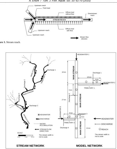
The mathematical model that was called SISMOD (Simple Stream Model), was realized according to specifications summarizes the paragraphs above. The first step of the realization was defining data structures that correspond to properties, physical components and environmental forcing related to a stream network. Those data structures are directly linked to model input data sets. The most basic data structure related to the stream network is a reach, which corresponds to a channel with unique geometrical properties. A reach can have several upstream reaches, but only one downstream reach. Other properties and environmental forcing are illustrated in Figure 1 and Figure 2.
The non-dispersive, steady state mass balance equation solved for any state variable along a reach is given by Eq. 1, where
( ) Q( ) ( )x Cx DIST DIST kC( )x 0
dx d x A
1
FLOW NO
FLOW+ + ⋅ =
+ ⋅ ⋅
− (Eq.1)
( )
x AC Q
DIST DIST DIST
flow
⋅
= (Eq.2)
x is the distance along the reach [L], A(x) is the cross-section area [L2], Q(x) is the flow rate along the reach [L3·T-1], C(x) is the concentration of the relevant water quality variable [M·L-3], DIST
STREAM REACH
Stream flow direction Upstream reach
Upstream reach Upstream reach
Point load
Diffuse load
without flow Downstream
reach
Diffuse load with flow
Figure 1. Stream reach.
15 km 9 km
HEADWATER 3
TRIBUTARY 2
M
A
IN
S
T
R
E
A
M
3 km
Discharge 4
Discharge 3 27 km
18 km
18 km HEADWATER 1
HEADWATER 2
TRIBUTARY 1 Discharge 1
9 km
6 km 1
2
3
4
5
6 7
8
HEADWATER
DISCHARGE
x REACH
MAIN STRE
AM
D
is
c
h
ar
ge
2
The stream width is not to scale Discharge 3
D
ischarge 4
D
ischarge 2
Discharge 1
MAIN S TREAM
M A
IN
S
T R E A M
MA IN S
TR EA
M
TR IBU
TA RY
1
TRIB UT
AR Y 2
HEADWATER
DISCHARGE SCALE
0 km 5 km 10 km
HEADWATER
DISCHARGE
WATER
STREAM FLOW DIRECTION ACCUMULATION
The stream width is not to scale
HEADWATER
DISCHARGE
MAIN STRE
AM
STREAM NETWORK MODEL NETWORK
Figure 2. Stream network and model network.
stream flow is expressed by Eq.2, where QDIST is the flow rate of the distributed source and CDIST is the concentration of the relevant water quality variable.
Depending on the water quality variable, the analytical solution of this equation may be simple or complex and even impossible for some cases. The distributed source terms (especially distributed loads with flow) make the analytical solution very complex or even impossible, when several water quality variables that depend on each other have to be expressed in form of a system of differential equations. Therefore, a semi-numerical approach is incorporated to solve the equations. Computational
points with equal distance to each other were defined along the stream reach as illustrated in the solution technique illustrated in Figure 3 is straightforward.
The hydraulic properties of the reach are assumed to be constant between two computational points; so that Eq 1 is reduced to Eq. 3; where U is the flow velocity [L·T-1], considering that the flow rate and the cross section area are constant and consequently, the flow rate can be moved to the left of the differential operator.
( )
x DIST DIST k C( )
xC dx
d
For each computational point, mass balance is formed between entering flow and distributed load WDIST [M·T-1] that is reduced to a point load and therefore Eq. 3 can be reduced to two equations; Eq. 4 and an algebraic mass balance equation (Eq. 6).
( ) ( )
U x C k x C dx
d = ⋅ (Eq.4)
Considering that distance (x) is equal to velocity (U) times travel time (t*) and velocity is constant, Eq. 4 can be rewritten as Eq. 5 (the differential form of the water quality routing equation) and the final model equations can be written as Eq. 6 and Eq. 7, where
( )
*( )
**Ct k Ct
dt d
⋅
= (Eq.5)
(
)
POINT W, DIST W, FINAL 1, -n
POINT DIST FINAL 1, -n FINAL 1, -n n,0 t
t* Q Q Q
W W Q
C C C
n + +
+ + ⋅
= =
=
(Eq.6)
( )
⎟⎟ ⎠ ⎞ ⎜⎜ ⎝ ⎛
⋅
=
∫
+=
=
* t
t
t t
* n,0
FINAL
n, f C , k Ct dt
C
1 n FINAL
n START
(Eq.7)
Cn-1,FINAL and Qn-1,FINAL are the concentration [M·L-3] and the flow rate [L3·T-1] just before the computational point n, Cn,0 is the concentration exactly on the computational point n, tn is the travel time passed until computational point n is reached and QW,DIST is the flow rate of the diffuse load, that is contributing to the flow rate of the stream [L3·T-1]. First, Eq. 6 (the mass balance equation) that is an
algebraic equation is solved at computational points to obtain Cn,0. Then Cn,0 is used to form Eq. 7 (the water quality routing equation) that is given in closed form. As seen above, Eq 6 also includes two additional terms; WPOINT that represents the total point load entering the computational point [M·T-1] and Q
W, POINT that represents the total flow rates of the point load [L3·T-1]. The indefinite integral term looks relatively easy to integrate; however, one should always keep in mind that water quality variables may depend on each other producing a more complex term k or a vector of k, if the modeller ends up in a system of differential equations as it was the case in this study.
The next step of the model realization was to decide on the contents of the water quality model in terms of water quality parameters. Usually four types of pollutants; conventional/collective organic parameters such as biochemical oxygen demand, total organic carbon; nutrients; heavy metals and toxic organics such as micro pollutants and pesticides. Modelling the behaviour of heavy metals necessitates a strong background in aquatic chemistry and modelling of toxic chemicals may be even more complex. It is doubtful that most of the users that may be at undergraduate level will have such a deep background in aquatic and organic chemistry. Another difficulty to incorporate this type of water quality parameters is that they have quite strong interactions among each other, and therefore, the model would be complex if a generally valid model construct is needed, or it would be narrowly specialized if few of them are added. In any case, the resulting model will be not suitable for educational/training purposes for those, who are having their first/preliminary training
Computational point n-1
Computational point n
DIST W, 0 n Q nQ Q= + ⋅
Δx
LREACH Δx
... ...
m L x= REACH
Δ Comp.points 2 to n-2
(n-2) x
Δ Comp.points n+2 to m Δx(m-n-1)
( )
DIST REACH DIST W,
FLOW NO DIST DIST REACH DIST
Q L
x Q
DIST C Q L
x W
⋅ Δ =
+ ⋅ ⋅ Δ =
DISTNO FLOW
LREACH
QDIST, CDIST
0
Q Qm=Q0+m⋅QDIST
Stream Flow Direction
Computational point n+1
Computational point m Computational
point 1 Computational
point 0
in water quality modelling. On the other hand, undergraduate level students in aquatic sciences, agriculture, fisheries, ecology, limnology, civil/hydraulic/environmental engineering and environmental sciences usually have sufficient background for understanding the key processes related to conventional/collective organic parameters and nutrients. Therefore; dissolved oxygen (O2), carbonaceous biochemical oxygen demand (CBOD), organic nitrogen (ORGN), ammonium nitrogen (NH4N), nitrite+nitrate nitrogen (oxidized nitrogen - NOXN), organic phosphorus (ORGP) and phosphate phosphorus (PO4P) were selected for the model as water quality variables. Following differential water quality routing equations analogous to Eq. 5, those include the key processes for the kinetics of these variables in streams, were defined for SISMOD:
[
]
[
]
rd r
* K CBOD L
dt CBOD
d =− ⋅ + (Eq. 8)
[ ] [ ] ([ ] [ ]) RESP PHOT NOXY SOXY O O K CBOD K dt O d 2 sat 2 a d
*2 =− ⋅ + ⋅ − − − + −
(Eq. 9)
[
]
nitr[
ORGN]
dt ORGN d
1,1
* =− ⋅
(Eq. 10)
[
]
nitr[
ORGN]
nitr[
NH4N]
dt NH4N d 2,2 1,2 * = ⋅ − ⋅
(Eq. 11)
[ ] nitr [NH4N] nitr [NOXN] dt NOXN d 3,3 2,3 * = ⋅ − ⋅
(Eq. 12)
[
]
[
]
ORGP phos dt ORGP d 1,1 * =− ⋅(Eq. 13)
[
]
[
]
[
]
PO4P phos ORGP phos dt PO4P d 2,2 1,2 * = ⋅ − ⋅(Eq. 14)
The terms in these equations are given in Table 1. Eq. 8 and Eq. 9 without its last four terms are the Streeter & Phelps equations (Streeter and Phelps, 1925) that formed the first mathematical stream water quality model in mid 1920s. Eq. 8 and Eq. 9 as they are formulated in SISMOD form an extended version of the Streeter & Phelps model. They represent the organic carbon and dissolved oxygen cycles. Eq. 10, Eq. 11 and Eq. 12 represent a simplified nitrogen cycle, where as Eq. 13 and Eq. 14 represent a simplified phosphorus cycle. As seen in those equations, a system of differential equations must be solved for each of these three cycles. The organic carbon and dissolved oxygen cycles depend on the nitrogen cycle because of the effect of nitrification process on dissolved oxygen. In order to simplify the solution, the inhibiting effect of severely depleted dissolved oxygen on nitrification is not incorporated directly into the nitrogen cycle. Instead SISMOD assumes that nitrification stops if dissolved oxygen concentrations decrease to 0.5 mg·L-1 or less. The
saturation concentration of dissolved oxygen was calculated according to (APHA, 1992).
The analytical solutions of Eq. 8 and Eq. 9 are given by Eq. 15 and Eq. 16 for aerobic sections of the stream. If dissolved oxygen decreases to 0.5 mg·L-1 or less, Eq. 17 is valid instead of Eq. 16. For the anaerobic sections of the stream, where dissolved oxygen is absolutely zero, Eq. 18 and Eq. 19 are valid instead of Eq. 15 and Eq. 16.
[ ] [ ]
(
)
(
(
*)
)
r r rd * r 02 1 exp K t
K L t K exp O
CBOD= ⋅ − ⋅ + − − ⋅ (Eq. 15)
[ ] [ ]( [ ]) ( ) ( ) ( ) ( ) [ ] ( ) ( ) [ ] ( ) [ ] ( ) ( ) ( ) ( ( ) ( )) ( ) ( ) ( ( )) ( ( )) a * a a * a a a * a rd * a * r r r a d * a r a d 0 2,2 * 2,2 2,2 2,3 0 2,2 * 2,2 1,1 * 1,1 1,1 2,2 2,3 1,2 0 * a * r r a d * a 0 2 sat 2 2 K SOXY t K exp 1 K R t K exp 1 K P t K exp 1 L t K exp t K exp K K K K t K exp 1 K K K NH4N nitr t nitr exp 1 nitr nitr ORGN nitr t nitr exp 1 nitr t nitr exp 1 nitr nitr nitr nitr 4.57 CBOD t K exp t K exp K K K t K exp O O O ⋅ ⋅ − − − ⋅ ⋅ − − − ⋅ ⋅ − − ⋅ ⎟ ⎟ ⎠ ⎞ ⎜ ⎜ ⎝ ⎛ ⎟⎟ ⎠ ⎞ ⎜⎜ ⎝ ⎛ ⋅ − ⋅ − − ⋅ ⋅ − + ⋅ − − ⋅ ⋅ − ⎟ ⎟ ⎠ ⎞ ⋅ ⎟ ⎟ ⎠ ⎞ ⎜ ⎜ ⎝ ⎛ − − ⋅ ⋅ ⎜ ⎜ ⎝ ⎛ + ⋅ ⎟ ⎟ ⎠ ⎞ ⎜ ⎜ ⎝ ⎛ − − ⋅ − − − ⋅ ⋅ − ⋅ ⋅ − ⋅ ⎟⎟ ⎠ ⎞ ⎜⎜ ⎝ ⎛ ⋅ − ⋅ − − ⋅ − − − ⋅ − =
(Eq. 16)
[ ] [ ] [ ]( )
(
)
(
) (
)
(
)
[ ](
)
(
)
( )(
(
) (
)
)
(
)
(
)
(
(
)
)
(
(
)
)
a * a a * a a a * a rd * a * r r r a d * a r a d 0 * a * r r a d * a 0 2 sat 2 2 K SOXY t K exp 1 K R t K exp 1 K P t K exp 1 L t K exp t K exp K K K K t K exp 1 K K K CBOD t K exp t K exp K K K t K exp O O O ⋅ ⋅ − − − ⋅ ⋅ − − − ⋅ ⋅ − − ⋅ ⎟ ⎟ ⎠ ⎞ ⎜ ⎜ ⎝ ⎛ ⎟⎟ ⎠ ⎞ ⎜⎜ ⎝ ⎛ ⋅ − − ⋅ − ⋅ − + ⋅ − − ⋅ ⋅ − ⋅ ⎟⎟ ⎠ ⎞ ⎜⎜ ⎝ ⎛ ⋅ − − ⋅ − ⋅ − − ⋅ − ⋅ − = (Eq. 17) [ ] [ ] [ ](
*)
START ANAEROBIC, * sat 2 a STARTANAEROBIC, K O t t
CBOD
CBOD= ⋅ ⋅ ⋅ −
(Eq. 18)
[ ]
O2 =0 (Eq. 19)The analytical solutions of the system of differential equations formed by Eq. 10, Eq. 11 and Eq. 12 are given by Eq. 20, Eq. 21 and Eq. 22 for aerobic sections of the stream. If dissolved oxygen decreases to 0.5 mg·L-1 or less or becomes zero, it is assumed that both nitrification and plant and phytoplankton activity stops and consequently none of the processes that are defined in the model consume ammonium nitrogen are active. In this case, Eq. 23 and Eq. 24 are used instead of Eq. 21 and Eq. 22. However, one must keep in mind that different values should be given to rate constants nitr1,1, nitr1,2 and nitr3,3 are valid for the anaerobic regions.
[
] [
]
(
*)
1,1
0 exp nitr t
ORGN
ORGN= ⋅ − ⋅ (Eq. 20)
[ ]
(
(
)
(
)
)
[ ](
*)
[ ]02 , 2 0 * 2 , 2 * 1 , 1 1 , 1 2 , 2 1,2 NH4N t nitr exp ORGN t nitr exp t nitr exp nitr nitr nitr NH4N ⋅ ⋅ − + ⋅ ⋅ − − ⋅ − ⋅ − =
[ ] ( ) ( ) ( ) ( ) [ ] ( ) ( ) ( )[ ] ( )
( 3,3 *)[ ]0
0 * 3 , 3 * 2 , 2 2 , 2 3 , 3 3 , 2 0 2 , 2 3 , 3 * 3 , 3 * 2 , 2 1 , 1 3 , 3 * 3 , 3 * 1 , 1 1 , 1 2 , 2 3 , 2 2 , 1 NOXN t nitr exp NH4N t nitr exp t nitr exp nitr nitr nitr ORGN nitr nitr t nitr exp t nitr exp nitr nitr t nitr exp t nitr exp nitr nitr nitr nitr NOXN ⋅ ⋅ − + ⋅ ⋅ − − ⋅ − ⋅ − + ⋅ ⎟ ⎟ ⎠ ⎞ − ⋅ − − ⋅ − ⎜ ⎜ ⎝ ⎛ − − ⋅ − − ⋅ − ⋅ − ⋅ =
(Eq. 22)
[ ]
(
(
)
)
[ ] [0 ]0* 1 , 1 1 , 1 1,2 NH4N ORGN 1 t nitr exp nitr nitr
NH4N=− ⋅ − ⋅ − ⋅ +
(Eq. 23)
[
] [
]
(
*)
3,3 0 exp nitr t
NOXN
NOXN = ⋅ − ⋅ (Eq. 24)
Similarly, analytical solutions for the phosphorus cycle are given by Eq. 25 and Eq. 26 for the aerobic regions and Eq. 26 and Eq. 27 for the anaerobic regions. The modeller must keep in mind that different values that should be given to rate constants phos1,1 and phos1,2 are valid for the anaerobic regions.
[ ] [ ]
(
*)
1,1 0 exp phos t ORGP
ORGP = ⋅ − ⋅ (Eq. 25)
[ ] ( ( ) ( ))[ ]
( 2,2 *)[ ]0
0 * 2 , 2 * 1 , 1 1 , 1 2 , 2 1,2 PO4P t phos exp ORGP t phos exp t phos exp phos phos phos PO4P ⋅ ⋅ − + ⋅ ⋅ − − ⋅ − ⋅ − =
(Eq. 26)
[ ]
(
(
)
)
[ ] [0 ]0* 1 , 1 1 , 1
1,2 exp phos t 1 ORGP PO4P
phos phos
PO4P =− ⋅ − ⋅ − ⋅ +
(Eq. 27)
The terms with subscript zero in Eq. 20 to Eq. 28 correspond to the concentrations exactly on location on the reach, where the calculation is initiated.
The independent variable used in Eq. 15 to Eq. 27 is the travel time t*. However, using the distance x instead of the travel time produces results that are more useful, since in most of the practical application, water quality profiles along the stream are of concern. Therefore, the travel times in those equations are written as distance over velocity and the values of the water quality variables are represented as a function dependent on the distance and velocity (and other model variables). Velocity is calculated using the Manning’s formula. Hydraulic calculations can be conducted for triangular, rectangular, trapezoidal and irregular cross-sections.
The final step of the model realization was to develop the main modelling software and the utility applications supporting it. All these software were developed according to open source philosophy in order to make them accessible to everybody who wants to use or modify them. Another advantage of this approach is that users will have the opportunity to observe how a model code looks like internally and can develop the basic ideas for their own researches in their later academic life or career. The main model was developed using Fortran 90. Fortran is the traditional programming language since late 1950s starting from IBM Fortran (Backus et al., 1956) in science and engineering. It is one of the most commonly used programming languages in science and engineering education (Brainerd et al., 1996). SISMOD is written using structured programming techniques. Special data structures were developed for model inputs and physical modelling environment.
The user has the option not to include nitrogen or phosphorus cycles into the simulation. SISMOD assumes that all the rate constants are entered for 20ºC water temperature. If the water temperature entered by the user is not 20ºC, then Arrhenius
Table 1. Terms used in model Equations
Term Description Unit
Ka Reaeration rate constant day-1
Kd Oxidation rate constant of carbonaceous BOD day-1
Kr Total carbonaceous BOD utilization rate constant (oxidation and settling) day-1
[ ]O2sat Saturation concentration of dissolved oxygen mg·L-1
Lrd Diffuse carbonaceous BOD load without flows mg·L-1day-1
PHOT Photosynthesis rate mg·L-1day-1
RESP Respiration rate mg·L-1day-1
SOXY Sediment oxygen demand mg·L-1day-1
NOXY Oxygen demand due to nitrification mg·L-1day-1
nitr1,1 Total organic nitrogen utilization rate constant (settling of particulate fraction, hydrolysis,
conversion to ammonium by bacteria) day
-1
nitr1,2 Conversion rate constant of organic nitrogen to ammonium nitrogen day-1
nitr2,2 Total ammonium nitrogen utilization rate constant (utilization by plants and
phytoplankton, nitrification)
day-1
nitr2,3 Nitrification rate constant day-1
nitr3,3 Total nitrate nitrogen utilization rate constant (utilization by plants and phytoplankton,
denitrification) day
-1
phos1,1 Total organic phosphorus utilization rate constant (settling of particulate fraction,
hydrolysis, conversion to phosphate phosphorus by bacteria) day
-1
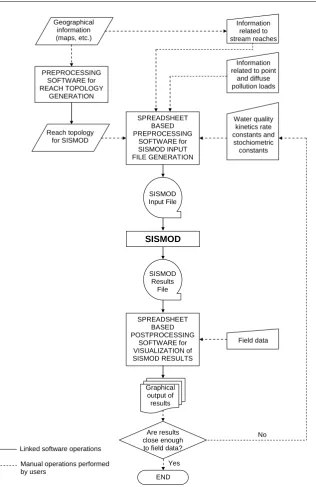
temperature correction equation is applied. Therefore, the user must also supply the temperature correction coefficients (θ) for each rate constant. The model inputs are plain text files that can be prepared with any text editor, alternatively, a spreadsheet based pre-processor developed under Microsoft Excel™. It is supplied with SISMOD and can be used to generate the model input file and run SISMOD. The post-processor integrated into the same spreadsheet application generates other spreadsheets that contain the model results and water quality profile plots along the reaches. These plots can also contain monitoring data in order to illustrate the model calibration process if necessary. Another spreadsheet-based utility that can generate profile plots from multiple model results to compare different simulations on the same stream is available as well. The flow diagram in Figure 4 illustrates the steps of using SISMOD and supporting utilities for a general model application.
Testing and Application of the Model
Testing is not only important in modelling but also important for software development. Any model code developed should undergo a quality control and quality assurance (QC/QA) process, before being released. Educational/training aimed software must also undergo a “usability test”, where the scientific consultants and the developer(s) should make sure that users with limited experience are able to use the software within a reasonable time of guided exercises and self-study.
SISMOD code was first compiled using different Fortran compilers and run. The results were compared to ensure that it is not affected by the difference of mathematical libraries included in different software development systems. Then, it was tested with many simple stream water quality examples from standard textbooks (Thomann and Mueller, 1987; Chapra, 1997) that were used for environmental/water quality modelling courses. The results indicated that SISMOD succeeded these tests. After these preliminary tests, SISMOD was given to undergraduate senior year (4th year) students taking the environmental modelling course as a basic tool for their term project, where a river that contains a main stream and several tributaries (usually around 15 reaches) was modelled. In these term projects, the students had to use all their knowledge on environmental engineering and basic modelling techniques to construct a model network from a given stream network, generate model inputs, run the model, analyze their outputs and generate materials for report writing. SISMOD was used for three years and four semesters (three fall semesters and a summer semester) by hundreds of students for such projects and appeared to be a successful educational/training tool.
Finally, SISMOD was tested on a “real-world” case. It was applied as a decision support system tool
for a water pollution control and watershed planning project the assessment of the river water quality and for comparing the benefits of different water control pollution measures for a 300 km long river that was intended as one of the future water resources for the mega city Istanbul (Erturk et al., 2007). SISMOD was calibrated, validated and then run monthly on a relatively complex model network with 6 headwaters, more than 80 reaches most of which have irregular cross-sections and numerous point (domestic and industrial wastewater discharges) and diffuse sources (land-based and atmospheric) for each month. Within the same study, it was also used to supply monthly water quality data for a reservoir water quality model developed by Erturk et al. (2008) for a planned reservoir, which will be constructed in the near future.
Results and Discussions
The product of this study is a training tool, which is water quality modelling software that is simple enough to be used effectively for educational/training purposes, but also comprehensive enough for institutional training that may cover real-world applications. The model was successfully tested and applied extensively for student training with considerable success. It was also applied as a decision support system tool to a study, where it underwent all the stages of traditional modelling such as verification, calibration and validation using real data and conducting real scenario analyses. Therefore, it can be considered as a verified model that is valid for similar river systems. The model source code, executable for Microsoft Windows operating system, example files and user documentation (in English and in Turkish) are available from the author. Since the model source code is available, it can be recompiled in any operating system and computer platform that have a Fortran 90&95 compiler available.
SISMOD software system could be further extended by a more user-friendly graphical interface with integrated help that assists the students during model setup process. This type of user interface can reduce errors, and even warn the trainees with limited experience and consequently make the training process more efficient. The postprocessor could be further developed to conduct data analysis on the results or generate maps according to user-defined criteria. SISMOD needs a runtime that rarely exceeds several seconds. Therefore it is also suitable for web based training. The executable can be installed on a web server and SISMOD can be made available to many trainees using a web-based user interface. Other ideas can also be realized, for example integrating SISMOD into special training packages such as game-based training software systems.
END PREPROCESSING
SOFTWARE for REACH TOPOLOGY
GENERATION Geographical information (maps, etc.)
No Reach topology
for SISMOD
SPREADSHEET BASED PREPROCESSING
SOFTWARE for SISMOD INPUT FILE GENERATION
Information related to stream reaches
Information related to point
and diffuse pollution loads
Water quality kinetics rate constants and
stochiometric constants
SISMOD Input File
SPREADSHEET BASED POSTPROCESSING
SOFTWARE for VISUALIZATION of SISMOD RESULTS
Field data
SISMOD
SISMOD Results
File
Graphical output of results
Are results close enough to field data?
Yes Linked software operations
Manual operations performed by users
Figure 4. Steps of using SISMOD and supporting utilities for a general model application.
used as a training tool for the first half of a water quality modelling course at undergraduate level or as a companion tool for water pollution control, water quality management or watershed planning courses. It can be used as an introductory training tool for institutional trainings in state offices that are responsible for topics related to water quality as well. However, it needs to be extended if the trainers decide to use it for training on more advanced modelling topics such as sensitivity/uncertainty analysis, optimization and numerical/dynamic modelling. In this case, further components and advanced versions of SISMOD should be developed.
Finally, besides being a training tool for
university students, SISMOD could also be used as a training tool for state institutes such as environmental ministries or environmental protection agencies. As stated before, two previous studies have proven that SISMOD can be applied to real cases. Therefore, it can be considered to be useful not only for training and education but also for screening of intermediate level of conventional stream water quality modelling purposes at state agencies.
Conclusion and Recommendations
study. Open source modelling software as well as several utilities were developed. The model was tested and then given to more than hundred students during an undergraduate environmental modelling course. The feedback from these students made clear that the concepts which the model is based on were found to be understandable and the use of the modelling tools was feasible on an undergraduate level one semester introductory environmental modelling course. Application of the model to a real modelling study has indicated that the model is reliable enough as a decision support system tool.
References
Ambrose, R.B., Wool, T. and Martin, J.L. 1993. WASP5, User’s manual. US Environmental Protection Agency, Environmental Research Laboratory, Athens, Georgia, GA, EPA/600/3-87-039.
APHA (American Public Health Association) 1992. Standart Methods for the examination of water and wastewater, 18th Ed., Washington D.C.
Backus, J.W., Beeber, R.J., Best, S., Goldberg, R., Herrick, H.L., Hughes, R.A., Mitchell, L.B., Nelson, R.A., Nutt, R., Sayre, D., Sheridan, P.B., Stern, H. and Ziller, I. 1956. The Fortan Automatic Coding System for IBM 704 EDPM, Applied Science Division abd Programming Research Dept., International Business Machines Corporation, New York, USA, 575 pp. Brainerd, W.S., Golberg, C.H. and Adams, J.C. 1996.
Programmer’s guide to F, Unicomp, Inc., Arizona USA.
Brown, C.L. and Barnwell, T.O. 1987. The enhanced stream water quality models QUAL2E and QUAL2E-UNCAS: Documentation and user Manual, US Environmental Protection Agency, Environmental Research Laboratory, Athens Georgia, EPA/600/3-87/007.
Chapra, S.C. 1997.Surface Water Quality Modelling, WBC/McGraw Hill, New York, USA.
Chwif, L., Paul, R.J. 2000. On simulation model complexity, In: J.A. Joines, R.R. Barton, K. Kang, and P.A. Fishwick (Eds.), Proceedings of the 2000 Winter Simulation Conference, Orlando: 449-455.
Cole, T.M. and Wells, S.A. 2002. CE-QUAL-W2 A two dimensional, laterally averaged, hydrodynamic and water quality model, Version 3.1. Instruction Report EL-2002-1, US Army Engineering and Research Development Center, Vicksburg, MS.
Environmental Laboratory 1995. CE-QUAL-RIV1: A dynamic, one-dimensional (longitudinal) water quality model for streams: User’s manual. Instruction Report EL-95-2, U.S. Army Engineer Waterways Experiment Station, Vicksburg, MS.
Erturk, A., Ekdal, A., Gurel, M., Yuceil, K. and Tanik, A. 2004. Use of Mathematical Models to Estimate the Effect of Nutrient Loadings on Small Streams, Fresenius Environmental Bulletin, 13(11b): 1350-1359.
Erturk, A., Gurel, M., Baloch, M.A., Dikerler, T., Ekdal, A., Tanık, A. and Şeker, D.Z. 2006. Applicability of modelling tools in watershed management for controlling diffuse pollution, Water Science &
Technology, 56(1): 147–154.
Erturk, A., Gurel, M., Ekdal, A., Tavsan, C., Seker, D.Z., Cokgor, E.U., Insel, G., Mantas, E.P., Aydin, E., Ozgun, H., Cakmakci, M., Tanik, A. and Ozturk, I. 2007. Estimating the Impact of Nutrient Emissions via Water Quality Modelling in the Melen Watershed, IWA 11th diffuse pollution conference and 1st meeting
of diffuse pollution and urban drainage specialist groups. 26-31 August, Belo Horizonte, Brazil. Erturk, A., Ekdal, A., Gurel, M., Zorlutuna, Y., Tavşan, C.,
Seker, D.Z., Tanik, A. and Ozturk, I. 2008. Application of Water Quality Modelling as a Decision Support System Tool for Planned Buyuk Melen Reservoir and Its watershed, In: İ.E. Gonenc, A. Vadineanu, C.P. Wolflin and R.C. Russo, (Eds.), Sustainable Use and Development of Watersheds, NATO Science for Piece and Security Series - C: Environmental Security, Springer, London: 227-242. Gurel, M., Salabas Cilek, A. and Gonenc, I.E. 2007. A
Database Management System for Model Coefficients Used in Modeling the Fate of Nutrients in Surface Waters, Clean-Soil, Air, Water, 35(6): 645-653. Jørgensen, S.E. 1996. State-of-the-art of ecological
modelling with emphasis on development of structural dynamic models. Ecological Modelling, 120: 75–96. Martin, J.L. and Wool, T. 2002. A dynamic one
dimensional model of hydrodynamics and water quality EPD-RIV1, Version 1.0. User’s manual, AScI Cooperation, Athens, Georgia.
Musselman, K.J. 1993. Guidelines for simulation project success. In: G. W. Evans, M. Mollaghasemi, E. C. Russell, and W.E. Biles (Eds.), Proceedings of 1993 Winter Simulation Conference, Institute of Electrical and Electronics Engineers, Piscataway, New Jersey: 58-64.
Pegden, C.D., Shannon, R.E. and Sadowski, R.P. 1995. Introduction to simulation using SIMAN, 2nd Ed., McGraw-Hill, New York, 839 pp.
Pidd, M. 1996. Five simple principles of modelling, In: J.M. Charnes, D.M. Morrice, D.T. Brunner and J.J. Swain (Eds.), Winter Simulation Conference, Institute of Electrical and Electronics Engineers, Piscataway, N.J.: 721-728.
Robinson, S. 1994. Successful simulation - A Practical Approach to Simulation Projects, McGraw-Hill Book Company Europe, Maidenhead, UK.
Salt, J.D. 1993. Keynote address: simulation should be easy and fun!, In: G.W. Evans, M. Mollaghasemi, E.C. Russell and W.E. Biles (Eds.), Winter Simulation Conference 1993, Institute of Electrical and Electronics Engineers, Piscataway, New Jersey: 1-5. Streeter, H.W. and Phelps, E.B. 1925. A Study of the
Pollution and Natural Purification of the Ohio River, III. Factors Concerning the Phenomena of Oxidation and Reaeration. Public Health Service, Bulletin No. 146. U.S., 75 pp.
Thomann, R.V., Mueller, J.A. 1987. Principles of Surface Water Quality Modeling and Control, Harper Collins publ., New York, 644 pp.