Re-Engineered Data Acquisition Model: A Statistical
Evaluation and Simulation
G. O. Uzedhe
Electronics DevelopmentInstitute, Awka, Federal Ministry of Science
and Technology, Nigeria
U. C. Ajuzie
Electronics DevelopmentInstitute, Awka, Federal Ministry of Science
and Technology, Nigeria
H. C. Inyiama
Electronics and Computer Department, Nnamdi AzikiweUniversity, Awka, Nigeria
A. C. O. Azubogu
Electronics and Computer Department, Nnamdi AzikiweUniversity, Awka, Nigeria
Abstract – This paper presents a statistical evaluation of a re-engineered data acquisition model for implementation. Data acquisition systems development is a dynamic field in industrial automation, especially in the search for low-cost and wide data coverage solutions. A re-engineered data acquisition model has been proposed and described by the authors, and can be implemented in diverse ways. This paper presents a statistical analysis of the model equation and performed a regressive calculation on a set of test signals for offset and gain determination. A simulation in SIMULINK showed that multi-parameter data can be acquired and stored in tables of records in a database for industrial process control and future operational behavioral predictions.
Keywords – Acquisition, Model, Linearization, Regression, Analysis.
I.
I
NTRODUCTIONThe design of a portable and robust Data Acquisition and Monitoring System (DAMS) is very important in the field of industrial automation. Such DAMSs are quite expensive and complex to develop due to diverse and sophisticated resources that are required. More so, their arrival at the market means that the users pay highly to acquire the necessary data system that can merely meet the need of the industry. Several remote solutions for data acquisition and monitoring have made their debut to the market but are still highly characterized with many drawbacks which do not amortize high cost, probably due to technologies employed in their development. For industries to survive and as well render good and quality services to their customers, low cost acquisition systems must be developed and deployed. Such low cost solutions must yield themselves to low maintenance cost, ease of use, short industry-to-market time while still maintaining the required data rate, accuracy, and precision that meet the industry standards.
Wireless [1] solution still remain the looking angle since it cuts off cost of running connection cables from one point to the other. Moreover, with today’s speed of wireless communication systems, their range of coverage, mobility, portability, and ease of use, it is clear that a wireless solution is a winner. Several wireless technologies exist [2], but the question is which one should be employed for a particular scenario or at best which combination should be used for optimal results? Must our solution be specific for each industrial area? Are multiplatform wireless solutions possible? The deployment of composite solutions that are able to acquire,
process, transfer data as well as monitor events in different application areas will be considered more encompassing. Uzedhe and Inyiama [3] presented a Re-Engineered Data Acquisition Model for Full Industrial Automation. They propose an all-inclusive data acquisition process by which machines, the environment and humans in the industry can be considered as part of an interactive system whose link must be maintained for true automation to be achieved. The model supports composite implementation for both wired and wireless multiplatform applications. This paper presents a statistical evaluation of the re-engineered model in order to establish its applicability in multi-parameter data acquisition environments.
II. R
EVIEW OFR
ELATEDW
ORKScollected directly at the RS-232 PC terminal through a Dynamic Link Library (DLL) function developed with Microsoft Visual C++ version 5. Edward et al [6] presented an embedded wireless data acquisition system model for wind tunnel applications as a replacement for conventional long wire connection systems. Wired data acquisition systems used in wind tunnel environments are susceptible to induced noise and requires multiple cable routes for data collection. In their work, an In-Model was developed and used to acquire field data and transferred to a remote computer through a wireless RF modem. The system was developed to use “Plug and Play/Test” concept with flexibility to support various signal inputs. It also show-cased miniaturize data acquisition system development for large application base. Yankee Environmental Systems [7] developed its YESDAS-2 data acquisition system for professional high availability data collection of environmental field parameters. The developer claimed a fast data processing, high conversion precision and large memory and I/O management at 12MHz. The YESDAS-2 system seems to be an ultimate winner for multichannel analogue input applications at good industrial standard resolution. However, its connection to Human-Machine Interfaces is through a compatible dial-up modem which limits its use for emerging remote Data Acquisition System (DAS). Ultimodule Inc. [8] developed an intelligent data acquisition system based on the Actel fusion Field Programmable Gate Array (FPGA) for building automation, advanced instrumentation, transport and automated control applications. The system promised flexibility for upgrading, migrating, and replacement especially when Fieldbus solutions are deployed. Juca et al [9] presented a low-cost concept for data acquisition system application in Decentralized Renewable Energy Plants (DREP). Their work decried the high cost of commercial DAS as a limitation to the spread of such systems in some parts of the world. They then proposed a
USB based DAS with dual clock operation philosophy for parallel information processing with different communication protocols. The work implements a DAS in which acquired data are stored in an external EEPROM and can be retrieved on a specified timely basis with the use of a Real Time Clock (RTC) connected to the EEPROM and a microcontroller through an I2C bus. Data communication to the computer and the RTC setting is done through a USB bus connection between the computer and the microcontroller. Their work also included interface to field devices for control and GSM/GPRS modem for network connectivity through the standard RS-232 protocol. K. Kalaitzakis et al [10] presented the development of a DAS for remote monitoring of renewable energy systems based on a Client/Server architecture without a physical connection to the monitored systems. In their work, vital signals at the remote station are acquired by a data acquisition unit and transmitted to collector unit through an RF wireless transceiver link and an RS-232 serial port. Several collection units then form an Ethernet or Internet network with a collection server through which client could have access to required information.
III. S
TATISTICALA
NALYSIS OF THER
E-ENGINEERED
M
ODELThe re-engineered model of [3] can be implemented in various ways in combinations of hardware and software propositions. However, it is noted that most data acquisition processes are statistical and require the collection of operational information with time. The acquired data Ad as presented in the re-engineered model Equation (1) is a composite sum of known and unknown variables and can only be determined with regression analysis. Details of the re-engineered model equation derivation can be found in [3].
A
d
1 N
n t1
t2
t a
nPn( )t d
= 1
R
r t1
t2
t b
rEr( )t d
= 1
L
l t1
t1
t c
lMl( )t d
= 1
Q
q t1
t2
t d
qDq( )t d
=
1
( )
Therefore, we represent the model equation in its statistical form as shown in equation (2).
Ad 1 n
i 1
t
j
Pi j =
= 1
r
i 1
t
j
Ei j =
= 1
l
i 1
t
j
Mi j =
= 1
q
i 1
t
j
Di j = =
2
( )
Where Pij represents the ith process value taken at the jth
time. Eij represents the ith environmental reading taken at
the jth time. Mij represents the ith machine emission taken
at the jth time. q represent the number of human health conditions taken into account at t time intervals and Dij
represents the ith health indicator taken at the jth time. Extracting the various industrial statistical components from the model, the process component, the environmental components, the machine component, and the human health components could be represented as given Equations (3) to (6) respectively.
f P( )
1 n
i 1
t
j P
ij = =
3 ( )
f E( )
1 r
i 1
t
j Eij = =
4
( )
f M( )
1 l
i 1 t
j Mij = =
5
f D( )
1 q
i 1
t
j Dij = =
6
( )
A. Linearization and Storage
In industrial data acquisition systems, the signal-flow processes are quite complex and un-predictable taking into account that field data are often accompanied by noise. Even when all control parameters (independent variables) remain constant, the resultant outcomes (dependent variables) vary. It is therefore necessary to pass the parameters through a process of linearization defined by Equation (7).
A
m
mA A
0( )
7
A = input variable, Am = output variable, A0 = signal offset, m = gain
From equation (7) the offset signal A0 represent the
initial input signal value at time t0 before measurements
are taken. This offset enables us to eliminate the undesired signal values at the output by way of subtraction. This offset may be a result of harmonic distortions introduced by the characteristics of the sensing devices. The gain m
helps to amplify or attenuate the signal as the case may be. When m is greater than one (m > 1) amplification is being applied, and when m is less than one (m < 1) attenuation is being applied. At unity gain (m = 1) the output signal is the same as the input signal.
Applying this linearization on each of the model equation components therefore further express the data sensing process to include signal gain and offset values as represented in Equations (8) through (11) thus:
f P( ) P
0
( )i1
n
i
1
t
j
pPij =
=
8
f E( ) E 0( )i
1
r
i
1
t
j
eEij =
=
9
f M( ) M
0 i( )
1 l
i 1
t
j
mMij
= =
10
( )
f D( ) D 0( )i
1 q
i 1
t
j
dD ij =
=
11 ( )
Where P0, E0, M0, D0 are offsets for each parameter type
and αp,αe, αm, αd are the desired gain factors. If we perform linearization on every data point acquired in time by the system, Equations (8) to (11) could be expanded and represented in their matrix form respectively in Equations (12) to (15) thus:
f P( )
P0 p P11
P0 p P21
_
_
_
P0 p Pi1
P0 pP12 ...
P0 pP22 ...
...
...
...
P0 pPi2 ...
P0 p P1.j
P0 p P2j
_
_
_
P0 p Pij
12 ( )
f E( )
E0 eE11
E0 eE21
_
_
_
E0 eEi1
E0 eE12...
E0 eE22...
...
...
...
E0 eEi2...
E0 eE1.j
E0 eE2j
_
_
_
E0 e Eij
13 ( )
f M( )
M
0 mM11
M
0 mM21
_ _ _ M0 mMi1
M
0 mM12 ...
M
0 mM22 ...
... ... ... M0 mMi2 ...
M
0 mM1.j
M
0 mM2j
_ _ _ M0 mMij
14
f D( )
D0 dD11
D0 dD21
_
_
_
D0 dDi1
D0 d D12 ...
D0 dD22 ...
...
...
...
D0 d Di2 ...
D0 d D1.j
D0 d D2j
_
_
_
D0 dDij
15
( )
These matrices of acquired signal points could then be multiplexed, concatenated and stored on a table representing a database of operational parameter values acquired over time. If for simplicity, each element of the
matrices is replaced in its simplest form, (i.e. X0 + αxXij is
replaced by Xij ) then the parameter database of acquired
data can be shown as represented in Equation (16).
Ad P11 P21 _ _ _ P i1
P12...
P22...
... ... ... P i2.... Pj P2j _ _ _ P ij E11 E21 _ _ _ E i1
E12...
E22....
... ... ... E i2... Ej E2j _ _ _ E ij M11 M21 _ _ _ M i1
M12...
M22...
... ... ... M i2... Mj M2j _ _ _ M ij D11 D21 _ _ _ D i1
D12...
D22...
... ... ... D i2... Dj D2j _ _ _ D ij 16 ( )
This process makes for easy data storage and retrieval as well as proper memory management. The acquired data, if stored in their raw values will require high precision data conversion process to store and retrieve them digitally. This also means that large amount of memory will be needed to store the data. When these data are to be transmitted and received over a wireless medium, more energy will be required to transmit the data bits. The linearization process employed could help to re-scale the signal level such that only a fraction of it, which represents the original signal value, is kept.
B. Determination of Offset and Gain
From the linearization process, consider a single input signal of each parameter group, that is, n = r = l = q = 1 and evaluating f(P), f(E), f(M), f(D) over a period of time,
t, then Equations (8) to (11) will becomes Equations (17) to (20) respectively thus,
f P( ) P 0
1 t
j
pP j =
17
( )
f E( ) E0
1 t
j
eEj=
18
( )
f M( ) M 0
1 t
j
mMj =
19
( )
f D( ) D 0
1 t
j
dDj =
20
( )
Equations (17) through (20) are in their regressive form and the best values of the offsets and gains are to be found
by a method of least squares (also known as regression analysis) to quantitatively estimate the trend of the outputs.
IV.
R
EGRESSIVEC
ALCULATION ANDS
IMULATION INMATLAB/SIMULINK
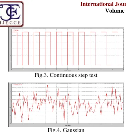
In order to simulate and evaluate the fit of the model, the sensor outputs applied to the model are set to continuous sinusoidal, ramp, step, and Gaussian noise test signals over a period of twenty seconds as shown in Fig 1, 2, 3 and 4 using Signal Builder source in SIMULINK. The equivalent signal values are then connected to the MATLAB workspace for regression analysis of Equations (17) through (20) to find the optimum values of the offsets
P0, E0, M0, D0 and gain αp,αe, αm, αd values for each group.
The resultant signal values are exported to MATLAB workspace to produced Tables of values for the offset and gain calculations.
Fig.1. Sinusoidal test
Fig.3. Continuous step test
Fig.4. Gaussian
A. Offset and Gain Calculation
In order to calculate the offset and gain values for each data group, the input signals are sampled at 1sec intervals for 20sec and then used to evaluate the respective
equations. Table 1 shows 20 sample values for the sinusoidal test signal. Thus, For Process Group using Equation (17):
Therefore,
20P0 + 28.9228αp = –29.7842 (21)
28.9228P0 + 312.6878αp = 92.1987 (22)
Solving equations (21) and (22) simultaneously yield
20
28.9228
28.9228
312.6878 P
0
p
29.7842
92.1987
P0 = -2.2114 and αp = 0.4994
The calculations were equally done for all other signal values and data groups to generate column 2 of Table 2. Using MATLAB Curve Fitting Tool (cftool) the R2 values and root mean squared errors for each signal type were found as shown in Table 2.
Table 1: Regression Analysis for Process Group
t (sec) P f(P) P2 P*f(P)
1 1.0000 -1.6548 1.0000 -1.6548
2 3.3511 -0.4792 11.2299 -1.6059
3 -1.9389 -3.1243 3.7593 6.0577
4 3.9389 -0.2254 15.5149 -0.8878
5 -3.7553 -4.0725 14.1023 15.2934
6 5.7553 0.6733 33.1235 3.8750
7 -3.7553 -4.0820 14.1023 15.3291
8 5.7553 0.6890 33.1235 3.9654
9 -1.9389 -3.1581 3.7593 6.1232
10 3.9389 -0.2810 15.5149 -1.1068
11 1.0000 -1.7505 1.0000 -1.7505
12 1.0000 -1.7936 1.0000 -1.7936
13 1.0000 -1.7936 1.0000 -1.7936
14 5.7553 0.6519 33.1235 3.7519
15 -1.9389 -3.1952 3.7593 6.1952
16 5.7553 0.6551 33.1235 3.7703
17 -3.7553 -4.1002 14.1023 15.3975
18 5.7553 0.6734 33.1235 3.8756
19 -3.7553 -4.0818 14.1023 15.3284
20 5.7553 0.6653 33.1235 3.8290
∑P = 28.9228 ∑f(P) = -29.7842 ∑P2 = 312.6878 ∑P*f(P) = 92.1987
Table 2: Offset and Gain values at 95% confidence bond
Equation Parameter Calculated Value R2 Value Root Mean Square Error Test Signal Type
P0, αp -2.2114, 0.4994 0.9996 0.04099 Sinusoidal
E0, αe -0.9392, 0.6692 0.9738 0.0455 Ramp
M0, αm -1.7247, 0.5042 0.9918 0.04207 Step
D0, αd -2.2697, 1.6245 0.9254 0.1237 Gaussian
Comparing these results showed that the sinusoidal test signal yields the optimal offset and gain values with the highest R2 value of 0.9996 and least root mean squared error of 0.04099 indicating a calculated gain of 0.4994 and an offset value of -2.2114. These values are then entered into a simulation model built in SIMULINK as shown in Figure 5 for the system output evaluation.
B. The Simulation Model in SIMULINK
variable u with i = 2 such that each parameter group is represented by two functions as shown in Fig. 5.
Fig.5. SIMULINK simulation
P
1
u
1
2
10 tan u( ),
P
2
u
10
cos u( )
u 4,
M1 u
1 2
0.05u 2.2 ,
M2 u
8 sin u( ) 5
D1 2 u u
1
2
5 ,
D2 u
5 0.1u
3
,
E
1 0.2u u 1 2
5
, E2 sin u( ) 5
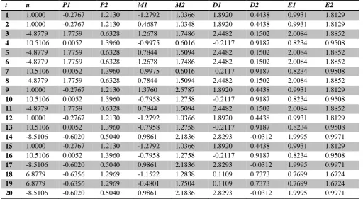
It should be noted that the functions define here may not be of any significant use to a desired application, but are used to demonstrate that signal of any nature can be acquired and stored in tables of records in a database for information retrieval. Table 3 shows data acquired using the defined functions acting on an input signal u for 20sec.
Table 3: Table of acquired data
t u P1 P2 M1 M2 D1 D2 E1 E2
1 1.0000 -0.2767 1.2130 -1.2792 1.0366 1.8920 0.4438 0.9931 1.8129
2 1.0000 -0.2767 1.2130 0.4687 1.0348 1.8920 0.4438 0.9931 1.8129
3 -4.8779 1.7759 0.6328 1.2678 1.7486 2.4482 0.1502 2.0084 1.8852
4 10.5106 0.0052 1.3960 -0.9975 0.6016 -0.2117 0.9187 0.8234 0.9508
5 -4.8779 1.7759 0.6328 0.7844 1.5094 2.4482 0.1502 2.0084 1.8852
6 -4.8779 1.7759 0.6328 1.2678 1.7486 2.4482 0.1502 2.0084 1.8852
7 10.5106 0.0052 1.3960 -0.9975 0.6016 -0.2117 0.9187 0.8234 0.9508
8 -4.8779 1.7759 0.6328 0.7844 1.5094 2.4482 0.1502 2.0084 1.8852
9 1.0000 -0.2767 1.2130 1.3760 2.5787 1.8920 0.4438 0.9931 1.8129
10 10.5106 0.0052 1.3960 -0.7958 1.2758 -0.2117 0.9187 0.8234 0.9508
11 -4.8779 1.7759 0.6328 0.7844 1.5094 2.4482 0.1502 2.0084 1.8852
12 1.0000 -0.2767 1.2130 -1.2792 1.0366 1.8920 0.4438 0.9931 1.8129
13 10.5106 0.0052 1.3960 -0.7958 1.2758 -0.2117 0.9187 0.8234 0.9508
14 -8.5106 -0.6020 0.5040 0.9861 2.1836 2.8293 -0.0312 1.9995 0.9971
15 1.0000 -0.2767 1.2130 -1.2792 1.0366 1.8920 0.4438 0.9931 1.8129
16 10.5106 0.0052 1.3960 -0.7958 1.2758 -0.2117 0.9187 0.8234 0.9508
17 -8.5106 -0.6020 0.5040 0.9861 2.1836 2.8293 -0.0312 1.9995 0.9971
18 6.8779 -0.6356 1.2969 -1.1522 1.2838 0.1109 0.7373 0.7699 1.6724
19 6.8779 -0.6356 1.2969 -0.4801 1.7504 0.1109 0.7373 0.7699 1.6724
20 -8.5106 -0.6020 0.5040 0.9861 2.1836 2.8293 -0.0312 1.9995 0.9971
V. R
ESULTS ANDC
ONCLUSIONThe data in Table 3 are clearly indexed in rows and columns and can be accessed with addresses of i x j values in memory. Though, the data shown are in their raw natural form (analogue representation), application of digital system implementation requires the conversion of these values to their digital format and make room for more flexibility in signal processing, data management, manipulation and system control. Application of the model equation to any multi-channel digital data acquisition system will provide access to timely industrial data. This paper has further shown that statistical analysis of multivariable data acquired from industrial operations with
the re-engineered model described in [3] will proffer a virile solution to all-inclusive data acquisition scenarios both in time and number of parameters measured.
R
EFERENCES[1] Hany Fouda (2006), “A review of wireless networks for remote monitoring and control applications”, Control Microsystems Inc. pp6.
[2] Dick Caro (2005), “Wireless Networks for Industrial Automation”, 2nd Edition, The Instrumentation, Systems and
Automation Society. pp25-50.
[4] P. Stephen Nischay and S. Latha (2012), “Design of DACS (Data Acquisition and Control System) using Linux”, International Journal of Emerging Technology and Advanced Engineering, Vol. 2 Issue 11, November 2012, www.ijetae.com [5] Y. Lan, X. Lin, M. F. Kocher, and W. C. Hoffmann (2007),
“Development of a PC-based Data Acquisition and Control System”, Agricultural Engineering International: the CIGR Ejournal, Vol. IX, August 2007.
[6] Edward Adock et al (2001), “An Embedded Wireless Data Acquisition System for Wind Tunnel Model Applications”, NASA Langley Research Center, Hampton.
[7] Yankee Inc. (2003), “Data Acquisition System Model YESDAS-2”, Yankee Environmental Systems, Inc. USA. http://www.yesinc.com
[8] Ultimodule (2005), “ Intelligent Data Acquisition System”, Ultimodule, Inc. http://www.ultimodule.com
[9] S. C. S.Juca, P. C. M. Carvalho and F. T. Brito (2011), “A Low Cost Concept for Data Acquisition Systems Applied to Decentralized Renewable Energy Plants”, Sensors 2011, 11, pp743-756. http://www.mdpi.com/journal/sensors.
[10] K. Kalaitzakis, E. Koutroulis and V. Vlachos (2003), “Development of a data remote monitoring of renewable energy systems”, Elsevier Ltd, Measurement 34 (2003) 75-83.
A
UTHOR’
SP
ROFILEProf. H. C. Inyiama
is a seasoned computer scientist and Engineer, with a wealth of experience in both industry and academics. He obtained his Bachelor’s Degree in Computer Technology from the University of Wales, University College of Swansea, U. K. (1978) before going over to the University of Manchester, Institute of Science and Technology (UMIST U.K.) for his Postgraduate Studies. He obtained his Ph.D. (UMIST) in December 1981. Since then he has held several posts nationally and internationally in the field of computer and information technology. He is duly registered professionally as both computer scientist and computer Engineer. His writing prowess derives from his wide professional exposure in academics and industry.
G. O. Uzedhe
is a Ph.D. student in the Department of Electronics and Computer Engineering, Nnamdi Azikiwe University Awka, Nigeria. His present research effort involves finding a low-cost solution for data acquisition systems in industrial automation environment and factory healthcare through wireless sensors. He is currently a Research Engineer and Digital Systems Developer at Electronics Development Institute (ELDI), Awka, Nigeria. He can be reached by Phone on +2348065720405 and through E-mail: [email protected]
A.C.O. Azubogu
hold B.Eng (Electronic Engineering) from the prestigious University of Nigeria, Nsukka; M.Eng (Telecommunication) from University of Port Harcourt and Ph.D (Signal Processing and Wireless Communication) from Nnamdi Azikiwe University, Awka. He is presently, a senior lecturer in the department of Electronic and Computer Engineering, Nnamdi Azikiwe University, Awka and the Associate Dean, Faculty of Engineering. He is also a member of the research team at the Wireless Communication Research Group. A.C.O Azubogu has over 20 papers published in reputable international journals. He is married with two beautiful children. He can be reached by phone on +2348059626829 and through E-mail: [email protected]
Engr. Ajuzie Uchechukwu
Chiemezuwoa
is Senior Research Engineer with Electronics Development Institute (ELDI) Awka, under the National Agency for Science and Engineering Infrastructure (NASENI), Nigeria. He obtained a B.Eng in Electrical/Electronics and Computer Engineering at Nnamdi Azikiwe University Awka, Anambra State, Nigeria in 2004, M.Eng in Electronics and Computer Engineering at the same university in 2009 and he is currently running his PhD program in Electronic and Computer engineeringin the same University. His research interest are Smart grid systems, security system automation, embedded control and communication systems with emerging wireless technologies. His contacts are Phone No: +2348030745870, E-mails: [email protected] or [email protected]