Development of a low-cost GPS/INS integrated system for tractor automatic navigation

(1)

Development of a low-cost GPS/INS integrated system for

tractor automatic navigation

Xiongzhe Han

1

_,

_{Hak-Jin Kim}

1*

_,

_{Chan Woo Jeon}

1

_,

_{Hee Chang Moon}

2

_,

_{Jung Hun Kim}

3

(1. Dept. of Biosystems and Biomaterials Engineering,College of Agriculture and Life Sciences, Seoul National University. Seoul 08826, Republic of Korea; 2. Unmanned Solutions Co., Seoul 06643, Republic of Korea;

3. R&D Institute, Tong Yang Moolsan Co., LTD, Chungcheongnam-do 32530, Republic of Korea)

Abstract: The use of low-cost single GPS receivers and inertial sensors for auto-guidance applications has been limited by their reduced accuracy and signal drift over time compared to real-time kinematic (RTK) differential GPS units and fiber-optic gyroscope (FOG) sensors. In this study, a prototype low-cost GPS/INS integrated system consisting of a triangle-shaped array of three Garmin 19x GPS receivers and an Xsens inertial measurement unit (IMU) to improve the accuracy of position and heading angle measured with a single GPS receiver was developed. A triangular algorithm that uses data collected from the three single GPSs mounted on the angular points of a triangular frame was designed. A sensor fusion algorithm based on the Kalman filter combining the GPS and IMU data was developed by integrating position data and heading angles of a triangular array of GPS receivers. The optimized values of two noise covariance matrixes (Q and R) for the Kalman filtering were determined using the Central Composite Design (CCD) method. As compared to the use of a single Garmin GPS receiver, use of the developed GPS/INS system showed improved accuracy performance in terms of both position and heading angle, with reductions in root mean square errors (RMSEs) from 2.7 m to 0.64 m for position and from 8.9º to 2.1º for heading angle. The accuracy improvements show new potential for agricultural auto-guidance applications.

Keywords: global positioning system, tractor, automatic navigation, sensor fusion, Kalman filter, inertial sensor, heading angle

DOI: 10.3965/j.ijabe.20171002.3070

Citation: Han X Z, Kim H J, Jeon C W, Moon H C, Kim J H. Development of a low-cost GPS/INS integrated system for tractor automatic navigation. Int J Agric & Biol Eng, 2017; 10(2): 123–131.

1 Introduction

The application of autonomous navigation to agricultural vehicles for precision farming is regarded as a successful example, with drastic potential improvements in agricultural mechanization. Main components required for automatic steering systems

Received date: 2016-11-28 Accepted date: 2017-02-20

Biographies: Xiongzhe Han, PhD, research interest: agricultural robots, Email: [email protected]; Chan Woo Jeon, PhD student, research interest: agricultural robots, Email: [email protected]; Hee Chang Moon,PhD, research interest: automotive engineering, Email: [email protected]; Jung Hun Kim, PhD, research interest: agricultural machinery, Email: [email protected].

*Corresponding author: Hak-Jin Kim, PhD, Associate Professor, research interest: precision agriculture. Department of Biosystems Engineering, College of Agriculture and Life Sciences, Seoul National University, Seoul 08826, Korea. Tel: 8228804604, Email: [email protected].

include various sensors to measure the position, heading angle, and inclination angle of a vehicle. Global Positioning Systems (GPSs) are presently used in many agricultural tasks[1-3]. Especially, GPS receivers with real-time kinematic differential corrections are frequently employed as navigation sensors in agricultural equipment, where they can provide centimeter-level accuracy[4,5]. However, the high cost of the real-time kinematic navigation sensors has limited the commercialization of autonomously guided agricultural machines such as tractors and combine harvesters[6,7]_.

(2)

124 March, 2017 Int J Agric & Biol Eng Open Access at https://www.ijabe.org Vol. 10 No.2 without the need for external references, thereby enabling

reliable position determinations. However, the INS sensor can suffer from signal drifts over time, and thus it is usually necessary to combine with GPS as a means to compensate for the errors[8-10]. The main challenge in developing a low-cost navigation system is the development of some methods to efficiently integrate complementary data of position and heading angle from the GPS and INS sensors to achieve high-accuracy position data.

Many researches focused on sensor fusion technology for agricultural vehicles have been conducted in recent years. Farrell et al.[11] proposed a real-time INS system aided by differential carrier phase GPS. The GPS aiding data were used to estimate errors in the INS state and to calibrate the inertia sensors, which improved the INS accuracy. Guo et al.[12] developed a GPS fusion system for positioning an off-road vehicle, consisting of a six-axis IMU and a Garmin GPS receiver. This fusion technology reduced the mean biases in the East and North axes to 0.48 m and 0.32 m, respectively. Guo et al.[13] developed a position-velocity-attitude (PVA) model-based fusion algorithm to provide dynamic positioning information for autonomous agricultural vehicles. The maximum positioning error of 0.3 m was measured for travel in open fields. Xiang et al.[14] tried to use a navigation system for remote sensing. The system was built using an autonomous UAV with an inertial sensor, a magnetometer, and a low-cost GPS receiver. A single board computer was used to provide continuous estimates of UAV position and attitude at 50 Hz using the sensor fusion techniques. Kownacki[15] mentioned a signal filtering problem with an accelerometer and a gyroscope. A Kaman filter was used for real-time filtering while a noise covariance matrix Q and a measurement noise covariance matrix R were determined. Gomez-Gil et al.[16] reported that implementation of the Kalman filter could reduce the quantization errors in the positioning of tractors equipped with low-cost GPS receivers by 43% as well as the standard deviation of the heading angle by 75%. Leung et al.[17] proposed an IKF (Integrated Kalman Filter) to estimate the vehicle dynamics using a GPS and an INS.

Simulation results showed that the proposed IKF was superior to conventional KF designs in estimating positions as long as the linear cornering coefficients are applicable to the vehicle model.

The goal of this research was to develop a navigation system that uses data collected from a triangle-shaped array of three low-cost single GPSs and an IMU, which is expected to solve the problem of low position accuracy that is obtained with a single GPS receiver. This paper describes the development of a positioning algorithm based on a sensor fusion technique that uses Kalman filtering while integrating signals measured with the GPS and IMU sensors.

2 Materials and methods

2.1 Triangular GPS positioning system

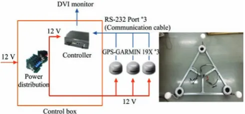
The Garmin GPS 19x HVS (Garmin International, Olathe, Kansas, USA)[18] units used in this study are relatively cheap single GPS receivers that include support for the Wide Area Augmentation System (WAAS)[19]_in the USA, thereby providing the position accuracy ranging from 4 m to 0.4 m. However, since the WASS service is not available in Korea, the Garmin receiver cannot receive signals from a satellite based augmentation system (SBAS) to compute and update its position to reach accuracy as that measured in the USA.

As shown in Figure 1, three Garmin-GPS 19x HVS receivers were installed on a triangular frame made of aluminum and each GPS unit was fixed 1 m from each of the other two. Each GPS receiver transmitted data at 10 Hz with a baud rate of 38 400 bps and received the ‘$GPRMC’ format data via the RS-232 communications, including information about latitude, longitude, heading, and velocity.

(3)

March, 2017Han X Z, et al. Development of a low-cost GPS/INS integrated system for tractor automatic navigation Vol. 10 No.2 125 In principle, the three GPS receivers form a triangle,

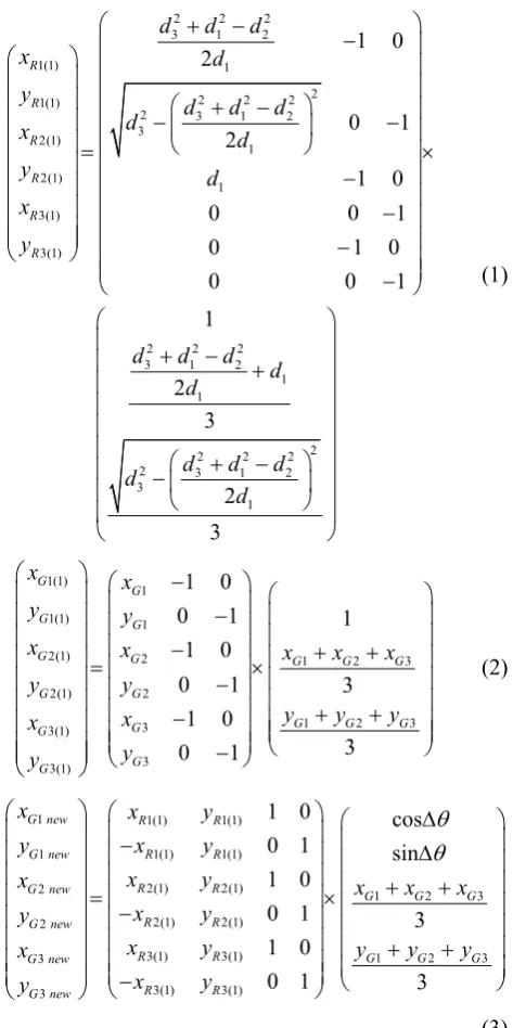
hereinafter called RDT (Range Data Triangle), and a virtual triangle called GDT (GPS Data Triangle) is generated using the actual data obtained from the three GPS receivers. The GDT data consisting of three different x-y coordinates are updated based on a comparison of geometrical points between the GDT and RDT. As shown in Figures 2a and 2b, the new coordinates (XRi(1), YRi(1)) and (XGi(1), YGi(1)) are calculated by changing the centroids of the RDT and GDT triangles to original point (0,0) using Equations (1) and (2). When the RDT performs a rotational motion, new corrected positions are determined under an optimized condition (Figure 2c). The optimized condition is obtained at a rotation angle that minimizes the distances between the points on the triangle using Equation (3).

a. Transformation of the RDT

b. Transformation of the GDT

c. Rotation of the RDT

Figure 2 Triangular error reduction method

2 2 2

3 1 2

1(1) 1

2

2 2 2

1(1)

2 3 1 2

3 2(1) 1 2(1) 1 3(1) 3(1) 1 0 2 0 1 2 1 0 0 0 1 0 1 0 + − − ⎛ ⎞ ⎜ ⎟ ⎜ ⎟ _⎛ ₊ ₋ _⎞ ⎜ ⎟ −_⎜ _⎟ − ⎜ ⎟₌ ⎝ ⎠ ⎜ ⎟ ₋ ⎜ ⎟ ⎜ ⎟ ₋ ⎜ ⎟ ⎜ ⎟ ₋ ⎝ ⎠ R R R R R R

d d d

x d

y _d _d _d

d

x _d

y _d

x y

2 2 2

3 1 2

1 1

2

2 2 2

2 3 1 2

3

1

0 0 1 1 2 3 2 3 ⎛ ⎞ ⎜ ⎟ ⎜ ⎟ ⎜ ⎟ ⎜ ⎟ ⎜ ⎟ × ⎜ ⎟ ⎜ ⎟ ⎜ ⎟ ⎜ ⎟ ⎜ ⎟ ⎜ ⎟ ⎜ ₋ ⎟ ⎝ ⎠ ⎛ ⎞ ⎜ ₊ ₋ ⎟ ⎜ ₊ ⎟ ⎜ ⎟ ⎜ ⎟ ⎜ ⎟ ⎜ _⎛ ₊ ₋ _⎞ ⎟ ⎜ _{− ⎜} _⎟ ⎟ ⎜ _⎝ _⎠ ⎟ ⎜ ⎟ ⎝ ⎠

d d d d d

d d d d d (1) 1(1) 1 1(1) ₁

2(1) 2 1 2 3

2(1) 2

1 2 3

3 3(1)

1 0

0 1 1 1 0

0 1 3

1 0 3 0 1 ⎛ ⎞ _⎛ ₋ _⎞ ⎜ ⎟ _⎜ _{⎟ ⎜}⎛ ⎞ ⎟ − ⎜ _{⎟ ⎜} ⎟ ⎜ ⎟ ⎜ _{⎟ ⎜} ₋ _⎟ + + ⎜ ⎟ ⎜ _{⎟ =}_⎜ _× ⎟ ⎜ ⎟ ⎜ ⎟ _⎜ ₋ ⎟ ⎜ ⎟ ⎜ _{⎟ ⎜} _⎟ ₊ ₊ − _⎜ _⎟ ⎜ ⎟ _⎜ _⎟ _⎜ _⎟ ⎜ ⎟ ⎜ ⎟ ₋ ⎝ ⎠ ⎜ _{⎟ ⎝} _⎠ ⎝ ⎠ G G G _G

G G G G G

G G

G G G

G G G G x _x y _y

x x x x x

y y

y y y

x x

y y

(2)

1 1(1) 1(1)

2(1) 2(1)

2 ₁

2(1) 2(1) 2 3(1) 3(1) 3 3(1) 3(1) 3

1 0 _cos 0 1 _sin 1 0 0 1 1 0 0 1 θ θ

⎛ ⎞ ⎛ ⎞ _Δ

⎜ ⎟ ⎜₋ ⎟ Δ ⎜ ⎟ ⎜ ⎟ ⎜ ⎟ ⎜ ⎟ ₊ ⎜ ⎟ =⎜ ⎟× − ⎜ ⎟ ⎜ ⎟ ⎜ ⎟ ⎜ ⎟ ⎜ ⎟ ⎜_⎜ ⎟_⎟ ⎜ ⎟ _⎝₋ _⎠ ⎝ ⎠

G new R R

R R

G new _G

R R G new R R G new R R G new

x x y

y x y

x y

x _x _x

x y y x y x x y y 2 3

1 2 3

3 3 ⎛ ⎞ ⎜ ⎟ ⎜ ⎟ ⎜ + ⎟ ⎜ ⎟ ⎜ ⎟ ⎜ + + ⎟ ⎜ ⎟ ⎝ ⎠ G G

G G G

x

y y y

(3) where, d1, d2, d3 are the lengths of the triangular edges;

Δθis the average rotation angle of the RDT triangle. 2.2 Kalman filtering

In principle, the Kalman filtering algorithm, which is commonly used as an optimal recursive computation of the least-squares algorithm, involves the use of a set of mathematical equations that implement a predictor- corrector type estimator based on the minimization of the estimated error covariance when the condition of a linear Gaussian system is met[20].

Figure 3 describes the filter in its original formulation, which includes measurements at discrete points in time. Ak is the transition matrix, which performs the prediction

model. Hk is the measurement sensitivity matrix that

(4)

126 March, 2017 Int J Agric & Biol Eng Open Access at https://www.ijabe.org Vol. 10 No.2 system sensors. $x_k and $

_ 1 k

x − are the priori and posteriori state estimate vectors, respectively. Q is the process noise covariance matrix of the prediction stage noise, which considers the weight of the process estimates. R is the observation noise covariance matrix of the update stage noise, which considers the degree of confidence in each of the measurements.

Figure 3 Diagram of Kalman filtering procedure[20] 2.3 Navigation system design with Kalman filter

To determine the real-time position and heading of a vehicle, a navigation system based on the use of multiple GPSs and an INS was developed. The major tasks of the navigation system design were to fuse data from the multiple sensors, which comprised a 3-axis rate gyroscope, a 3-axis accelerometer, and the triangular GPS system. In principle, the INS uses the gyroscope and accelerometer to provide data on position and attitude of

the vehicle at a high frequency. However, the error of this data gradually increases owing to the accumulation of error from the accelerometer and rate gyroscope measurements. On the other hand, GPS can provide accurate positioning for long periods, but the signals can be easily influenced owing to outside interfering effects such as buildings and trees. To use both GPS and INS in a way that makes up for each technique’s disadvantages, a sensor fusion algorithm based upon Kalman filtering was developed. The corrected information was estimated through the integration of relative positioning and absolute positioning to improve the positioning accuracy of the system as shown in Figure 4.

Figure 4 Concept of the sensor fusion algorithm

Nine variables were selected to build a non-linear state equation representing the 3D system model (Guo et

al. [12]) of a vehicle as described in Equation (4).

0 0 0 1 0 0 0 0 0 0 0 0 0 1 0 0 0 0 0 0 0 0 0 1 0 0 0 0 0 0 0 0 0 0 0 0 0 0 0 0 0 0 0 0 0 0 0 0 0 0 0 0 0 0 0 0 0 0 0 0 0 0 0 0 0 0 0 0 0 0 0 0 0 0 0 0 0 0 0 0 0

φ φ

θ θ

ψ ψ

⎡ ⎤ _{⎡ ⎤}

⎡ ⎤

⎢ ⎥ _{⎢ ⎥}

⎢ ⎥

⎢ ⎥ _{⎢ ⎥}

⎢ ⎥

⎢ ⎥ _⎢

⎢ ⎥

⎢ ⎥ _⎢

⎢ ⎥

⎢ ⎥ _⎢

⎢ ⎥

⎢ ⎥ _⎢

⎢ ⎥

⎢ ⎥ = _⎢

⎢ ⎥

⎢ ⎥ _⎢

⎢ ⎥

⎢ ⎥ _⎢

⎢ ⎥

⎢ ⎥ _⎢

⎢ ⎥

⎢ ⎥ _⎢

⎢ ⎥

⎢ ⎥ _⎢

⎢ ⎥

⎢ ⎥ _⎢

⎣ ⎦

⎢ ⎥ ⎣ ⎦

⎣ ⎦ & & & & & & & & &

x

x y

y

z _z

x x

y y

z z

P _P

V V

1 0 0 1 0 0 0 0 0

0 1 0 0 0 0 0 0 0

0 0 1 0 0 0 0 0 0

0 0 0 cos cos sin cos cos sin sin sin sin cos sin cos 0 0 0

0 0 0 sin cos cos cos sin sin sin cos sin sin sin cos 0 0 0

0 0 0 sin cos sin cos cos 0 0 0

0 0 0 0 0 0 1 sin tan cos t

ψ θ ψ φ ψ θ φ ψ φ ψ θ φ

θ θ φ θ φ

φ θ φ

⎥ ⎥ ⎥ ⎥ + ⎥ ⎥ ⎥ ⎥ ⎥ ⎥ ⎥

− + +

+ − +

−

0 0 0

an

0 0 0 0 0 0 0 cos sin

0 0 0 0 0 0 0 sin / cos cos / cos

θ ω

φ φ _ω

φ θ φ _{θ ω}

⎡ ⎤

⎡ _{⎤ ⎢ ⎥}

⎢ _{⎥ ⎢ ⎥}

−

⎢ _{⎥ ⎢ ⎥}

⎣ _{⎦ ⎣ ⎦}

x

y

x

y

z

a a a

(5)

where, =[ , , , , , , , , ]φ θ ψ T

k x y z x y z k

x P P P V V V is a state vector

at time tk; [ , , ]P P Px y z kT, [ , , ] T x y z k

V V V , [ , , ]φ θ ψ T

k are the position, velocity and attitude vectors of the vehicle in the navigation coordinate frame; [ , , ]T

x y z k

a a a , [ ,ω ω ω, ]T x y z k are the vectors of vehicle acceleration and angular rate in the body coordinate frame.

Assuming that the vehicle travels in a 2D field, the system model was simplified from a 3D space to a 2D space allowing reduction of the number of state variables to 5. A modified nonlinear state equation including this reduced set of variables was established as described in Equation (5).

0

0 0 1 0 0 1 0 0 0 0

0

0 0 0 1 0 0 1 0 0 0

0 0 0 0 0 0 0 cos sin 0 0 0 0 0 0 0 0 sin cos 0

0 0 0 0 0 0 0 0 0 1

ψ ψ ψ ψ ω ψ ⎡ ⎤ ⎡ ⎤⎡ ⎤ ⎡ ⎤⎡ ⎤ ⎢ ⎥ ⎢ ⎥⎢ ⎥ ⎢ ⎥⎢ ⎥ ⎢ ⎥ ⎢ ⎥⎢ ⎥ ⎢ ⎥⎢ ⎥ ⎢ ⎥=⎢ ⎥⎢ ⎥+⎢ ⎥⎢ ⎥ ⎢ ⎥ ⎢ ⎥⎢ ⎥ ⎢ ₋ ⎥⎢ ⎥ ⎢ ⎥ ⎢ ⎥⎢ ⎥ ⎢ ⎥⎢ ⎥ ⎢ ⎥ ⎢_⎣ ⎥_⎦⎢ ⎥_{⎣ ⎦} ⎢_⎣ ⎥_{⎦⎣ ⎦}⎢ ⎥ ⎣ ⎦ & & & & & x x y y x x x y y y x z P P P P V a V V a V V (5) To allow its application in the Kalman filter algorithm, the state equation of the system model was simplified as shown in Equation (6).

1

1 0 0 0 0

0 1 0 0 0

0 0 1 0 0 ( sin cos ) 0 0 0 1 0 ( cos sin ) 0 0 0 0 1

0 0 0 0 0 1

ψ ψ ψ ψ ω + Δ ⎡ ⎤

⎢ _Δ ⎥

⎢ ⎥

⎢ Δ − − ⎥

=_⎢ _⎥ +

Δ −

⎢ ⎥

⎢ _Δ ⎥

⎢ ⎥

⎣ ⎦

x y

k k k

x y

z t

t

t a a

x x w

t a a

t

(6) where, wk is the Gaussian white noise source for the state

equation; xk is the state vector at time tk; Δt is the time

step.

GPS data were used to determine a measurement model from Equation (7) based on position, velocity, and heading angle in the measurement process.

0.5 0.5

1 0 0 0 0 0

0 1 0 0 0 0

0 0 0 0

0 0 0 0 1 0

k k k

z x v

⎡ ⎤ ⎢ ⎥ ⎢ ⎥ =_⎢ _⎥ + ⎢ ⎥ ⎣ ⎦ (7)

where, =[ , , , ]ψ T

k N E k

z P P V is a measurement vector

from the GPS; PN, PEare the north and east coordinates,

respectively; V and ψ are the velocity and yaw angles

measured with the GPS; vk is the Gaussian white noise

source for the state equation of the measurement model.

2.4 Optimization of noise covariance matrices Assuming that all state variables are statistically independent and that the covariance matrices are time-invariant, the covariance Q and R matrices can be expressed as Equation (8). Because a preliminary experiment showed that the elements a, b, c, and d did not show significant effects on the outputs of the estimation algorithm, a=b=0.001, c=0.1 and d=0.005 were chosen as constant values in the noise covariance matrix.

1

2

3

4 0 0 0 0 0

0 0 0 0 0

x x x x a b ⎡ ⎤ ⎢ ⎥ ⎢ ⎥ ⎢ ⎥ = ⎢ ⎥ ⎢ ⎥ ⎢ ⎥ ⎢ ⎥ ⎢ ⎥ ⎣ ⎦ Q , 5 6 0 0 0

0 0 0

0 0 0 x x c d ⎡ ⎤ ⎢ ⎥ ⎢ ⎥ = ⎢ ⎥ ⎢ ⎥ ⎣ ⎦ R (8)

Simulations were conducted to determine optimal values of the variables [x1, x2, x3, x4] in Q, and of the variables [x5, x6] in R. The central composite design (CCD) method was then performed based on the output of two position root mean square errors (RMSEs) , i.e., Y1 and Y2, obtained with the developed system following along a straight path and a curved path, respectively, and heading angle RMSE (Y3). The RMSEs were calculated using Equation (9). Forty-six simulation trials with different parameter values were selected based on a six-factor, three-level experimental design. The statistical program Minitab (Ver17.1.0) was used to determine the optimal values. Regression analysis was used to investigate and model the relationships between the six factors and measured RMSEs.

2 2

1 1

[( ) ( ) ]

N

i d i d

RMSE x x y y

N

=

∑

− + −

(9)

where, (xi, yi) is estimated position based on fusion

algorithm; (xd, yd) is desired position based on RTK-GPS;

N is the number of data.

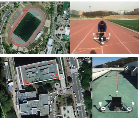
2.5 Paved road tests for system evaluation

(6)

128 March, 2017 Int J Agric & Biol Eng Open Access at https://www.ijabe.org Vol. 10 No.2 Sciences Building. The running track prepared in the

stadium comprised a 90 m straight path followed by a 50 m curved path. The paths of the building roof were composed of three straight paths, i.e., a path of 70 m and the other two paths of 30 m. The traveling speed was maintained at approximately 3 km/h during the test. For comparison with the developed positioning system based on the triangular GPS and IMU system, a Novatel FlexPak-G2 real-time kinematic global positioning system (RTK-GPS) was used as a reference system to measure real positions during the tests. The reference system transmitted position data at 10 Hz with the data rate of 115 200 bps, providing the performance of position accuracy to within 2 cm. The dynamic trajectory of the vehicle obtained from the integrated system at a sampling rate of 20 Hz was compared to the reference path. The RMSEs obtained from the road tests were used to evaluate the differences between the points estimated using the proposed algorithm and the reference path points.

Figure 5 Evaluation tests run on a running track (top) and a building roof (bottom)

3 Results and discussion

3.1 Optimization of low-cost GPS system parameters Using the CCD experimental method, the parameters related to position estimation within the noise covariance matrices Q and R were optimized. The results of ANOVA analysis of the significance of the six factors x=[x2, x3, x3, x4, x5, x6] on the RMSEs of the straight and curved paths showed that all of the six factors were

significant variables affecting the RMSE values, i.e., p<0.0001 for each of the six factors.

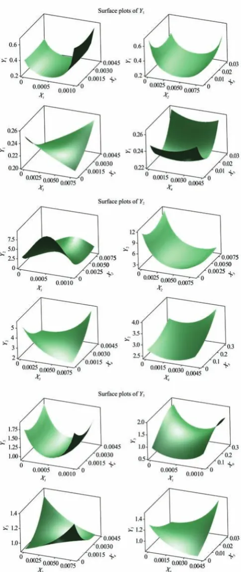
Figure 6 shows the surface plots of Y1, Y2 and Y3, (i.e., RMSEs measured at straight path position, curved path position, and heading angle, respectively) with respect to part of the six factors. The results of ANOVA analysis showed that there were significantly linear relationships between the six factors and RMSE values measured at the straight path (R2=0.86, p<0.0001). The regression equation for Y1 was obtained as follows:

1 [ 2820 204 27 62 3 8.36]

3094401 146827 2624 931 10907 5591 0 45348 400 991 2757 2090

0 0 357 2973 150 25

0 0 0 4151 284 27

0 0 0 0 351 163

0 0 0 0 0 65.4

1.755

= − − − − +

− − −

⎡ ⎤

⎢ ₋ ₋ ⎥

⎢ ⎥

⎢ − ⎥

⎢ ₋ ₋ ⎥

⎢ ⎥

⎢ ₋ ⎥

⎢ ⎥

⎣ ⎦

+

T

Y X

XX

(10)

In addition, it was found that there were significantly linear relationships between six factors and RMSE measured at the curved path (R2_=0.88,_p_{<0.0001). The} regression equation for Y2 was:

2 [ 2820 204 27 62 3 8.36]

1105518 119048 27125 39548 32196 1558 0 15701 4737 10301 304 739 0 0 45609 23609 1775 273

0 0 0 118015 2959 247

0 0 0 0 2191 85

0 0 0 0 0 14

2.47

= − − − − +

− − −

⎡ ⎤

⎢ ₋ ₋ ₋ ⎥

⎢ ⎥

⎢ − ⎥

⎢ ₋ ⎥

⎢ ⎥

⎢ ₋ ⎥

⎢ ⎥

⎣ ⎦

+

T

Y X

XX

(11) Finally, significantly linear relationships between six factors and heading RMSEs were obtained (R2=0.83, p<0.0001). The regression for Y3was:

3 [ 6079 396 139 328 100.9 6.12] 6031438 129988 4317 83899 7207 1347

0 36330 3362 5466 180 457 0 0 22077 34873 5765 457

0 0 0 128070 9971 1189

0 0 0 0 1349 155

0 0 0 0 0 5.33

3.085

= − − − − − +

− −

⎡ ⎤

⎢ ₋ ₋ ⎥

⎢ ⎥

⎢ − − ⎥

⎢ ₋ ⎥

⎢ ⎥

⎣ ⎦

+

T

Y X

XX

(7)

March, 2017Han X Z, et al. Development of a low-cost GPS/INS integrated system for tractor automatic navigation Vol. 10 No.2 129

Figure 6 Surface plots of RMSEs of straight (Y1), curved (Y2), and heading angle (Y3) with respect to part of six factors

Optimized values were determined using the 3D surface plots for any of pair factors by finding minimal values to satisfy with all of the output RMSEs (Y1, Y2, and

Y3). Equation (13) shows the results of the response optimization of noise covariance matrices Q, R based on the output RMSEs Y1-Y3.

=

Q

0.00003321 0 0 0 0 0

0 0.00697 0 0 0 0

0 0 0.00461 0 0 0

0 0 0 0.00186 0 0

0 0 0 0 0.001 0

0 0 0 0 0 0.001

⎡ ⎤

⎢ ⎥

⎣ ⎦

0.0245636 0 0 0

0 0.206092 0 0

0 0 0.1 0

0 0 0 0.005

⎡ ⎤

⎢ ⎥

=

⎢ ⎥

⎣ ⎦

R (13)

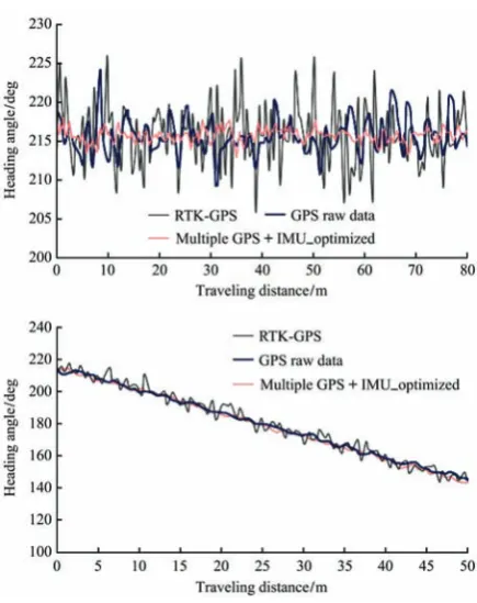
3.2 Results of system evaluation on paved roads Figure 7 compares the position data obtained at the straight and curved paths from the paved road tests. The blue path represents the raw data of a single GPS unit and the red path represents the data obtained using the developed positioning system. The gray path represents the data from the reference with the RTK-GPS receiver. The positions estimated by the proposed GPS-INS sensor system after applying the algorithm were improved as compared to those measured by the single GPS receiver. Furthermore, regardless of whether the position was on a straight or curved path, the corrected heading angles became stable, showing relatively consistent values (Figure 8). Figure 9 compares RMSE performance for the single GPS receiver, multiple GPSs receivers and the proposed GPS/INS system in terms of position and heading angle. The position RMSE of the straight path was reduced from 2.64 m to 0.77 m, and that of the curved path was improved from 1.56 m to 0.43 m.

(8)

130 March, 2017 Int J Agric & Biol Eng Open Access at https://www.ijabe.org Vol. 10 No.2

Figure 7 Position results of single GPS receiver, proposed multi-GPS/INS system, and reference system measured at straight

(top) and curved paths (bottom)

Figure 8 Heading results of single GPS receiver, proposed multi-GPS/INS system, and reference system measured at straight

(top) and curved paths (bottom)

Figure 9 Comparison of RMSEs of a single GPS receiver, multi GPS receivers, and the proposed multi-GPS/INS systems

Figure 10 Comparison of a single GPS and proposed multi-GPS/INS system with respect to absolute position (top) and

lateral deviation (bottom)

(9)

March, 2017Han X Z, et al. Development of a low-cost GPS/INS integrated system for tractor automatic navigation Vol. 10 No.2 131

4 Conclusions

In this study, a low-cost GPS/INS integrated system for an autonomously guided tractor was proposed. A Kalman filtering based triangular positioning algorithm that uses data collected from three single GPS receivers to improve the positioning accuracy was developed. A basic idea was that corrected information is estimated based on the integration of relative and absolute positioning data. The noise covariance matrices Q and R for the Kalman filter were determined by CCD experimental method. Compared to the use of a single Garmin GPS receiver, the test results of the developed GPS/INS system showed that the accuracy performance in terms of both position and heading angle was improved, with reductions in RMSE from 2.7 m to 0.64 m for position and from 8.9º to 2.1º for heading angle, respectively.

Acknowledgments

This research was supported in part by the Korea Evaluation Institute of Industrial Technology (10049017, 2014-2016), and Agricultural Robotics and Automation Research Center, Korea Institute of Planning and Evaluation for Technology in Food, Agriculture, Forestry and Fisheries (714002-7, 2014-2016), Republic of Korea.

[References]

[1] Slaughter D C, Giles D K, Downey D. Autonomous robotic weed control systems: A review. Computers and Electronics in Agriculture, 2008; 61(1): 63–78.

[2] Zhang N, Wang M, Wang N. Precision agriculture: a worldwide overview. Computers and Electronics in Agriculture, 2002; 36(2): 113–132.

[3] Auernhammer H. Precision farming: the environmental challenge. Computers and Electronics in Agriculture, 2001; 30(1): 31–43.

[4] Keicher R, Seufert H. Automatic guidance for agricultural vehicles in Europe. Computers and Electronics in Agriculture, 200; 25(1): 169–194.

[5] Mizushima A, Noguchi N, Ishii K, Terao H. Development of navigation sensor unit for the agricultural vehicle. In Proceedings of the Advanced Intelligent Mechatronics, 2003; 1067–1072.

[6] Li M, Imou K, Wakabayashi K, Yokoyama S. Review of research on agricultural vehicle autonomous guidance. Int J

Agric & Biol Eng, 2009; 2(3): 1–16.

[7] Shearer S A, Pitla S K, Luck J D. Trends in the automation of agricultural field machinery. In Proceedings of the 21st Annual Meeting of the Club of Bologna. Italy, 2010.

[8] Cappelle C, Pomorski D, Yang Y. GPS/INS data fusion for land vehicle localization. In Proceedings of the Computational Engineering in Systems Applications, 2006; 1: 21–27.

[9] Dissanayake G, Sukkarieh S, Nebot E, Durrant-Whyte H. The aiding of a low-cost strapdown inertial measurement unit using vehicle model constraints for land vehicle applications. IEEE Transactions on Robotics and Automation, 2001; 17(5): 731–747.

[10] Noureldin A, Karamat T B, Eberts M D, El-Shafie A. Performance enhancement of MEMS-based INS/GPS integration for low-cost navigation applications. IEEE Transactions on Vehicular Technology, 2009; 58(3): 1077–1096.

[11] Farrell J A, Givargis T D, Barth M J. Real-time differential carrier phase GPS-aided INS. IEEE Transactions on Control Systems Technology, 2000; 8(4): 709–721.

[12] Guo L, Zhang Q, Feng L. A low-cost integrated positioning system of GPS and inertial sensors for autonomous agricultural vehicles. In Proceedings of the American Society of Agricultural Engineers, 2003; Paper No. 033112. [13] Guo L, Zhang Q. A low-cost integrated positioning system

for autonomous off-highway vehicles. Journal of Automobile Engineering, 2008; 222(11): 1997–2009.

[14] Xiang H, Tian L. Development of a low-cost agricultural remote sensing system based on an autonomous unmanned aerial vehicle (UAV). Biosystems Engineering, 2011; 108(2): 174–190.

[15] Kownacki C. Optimization approach to adapt Kalman filters for the real-time application of accelerometer and gyroscope signals’ filtering. Digital Signal Processing, 2011; 21(1): 31–140.

[16] Gomez-Gil J, Ruiz-Gonzalez R, Alonso-Garcia S, Gomez-Gil F J. A kalman filter implementation for precision improvement in low-cost GPS positioning of tractors. Sensors, 2013; 13(11): 15307–15323.

[17] Leung K T, Whidborne J F, Purdy D, Barber P. Road vehicle state estimation using low-cost GPS/INS. Mechanical Systems and Signal Processing, 2011; 25(6): 1988–2004.

[18] Garmin GPS 19x HVS technical specifications. http://www.fo ndriest.com/pdf/garmin_19xhvs_spec.pdf. [19] Enge P, Walter T, Pullen S, Kee C D, Chao Y C, Tsai Y J.

Wide area augmentation of the global positioning system. In Proceedings of the IEEE, 1996; 84(8): 1063–1088.