Web Ecology 9: 58–67.
There is currently an increasing need to monitor and as-sess regional, continental and global spatial processes in a changing inter-connected world (Johnston et al. 2002). Consequently, researchers are beginning to integrate data on a regional or global scale with local studies in order to develop multi-hierarchical frameworks that address the complexity of environmental and social systems (Good-child 2001, Brown et al. 2002). In addition, the inclu-sion of the spatial vector in scientific studies, supported by Geographic Information Systems (GIS), is required by land-planners and administrators in order to generate supporting management tools. To go beyond non-spatial approaches, predictive modelling of spatial patterns on all scales is one of the main topics of location-related sciences such as biogeography, climatology, hydrology, ecology and landscape ecology (Haines-Young et al. 1993, Maidment and Djokic 2000, Austin 2002). In addition, the quality of predictions about the effect of global change on features
such as biodiversity, water availability, erosion processes and others are also determined by the accuracy of the pre-dictive tools (Thuiller 2003). Consequently, the evalua-tion of predictive tools is essential for the improvement of results and subsequent management strategies.
There is an extensive list of spatially predictive ap-proaches, models and techniques. According to Guisan and Zimmermann (2000), three large groups of predictive models can be recognised: 1) analytical or mathematical, such as the general logistic growth equation, 2) mechanis-tic or process-oriented models based on the theoremechanis-tical cor-rectness of the predicted response, and 3) statistical models based on the correlations between predictors and response variables, although some authors maintain that this distinc-tion is often unclear (Peters 1991). In terms of statistical models, many techniques have been applied to spatial data: regression analysis (MacNally 2000), classification and or-dination techniques such as regression trees and various
Comparing regression methods to predict species richness
patterns
David Nogués-Bravo
Nogués-Bravo, D. 2009. Comparing regression methods to predict species richness patterns. – Web Ecol. 9: 58–67.
Multivariable regression models have been used extensively as spatial modelling tools. However, other regression approaches are emerging as more efficient techniques. This paper attempts to present a synthesis of Generalised Regression Models (Generalized Linear Models, GLMs, Generalized Additive Models, GAMs), and a Geographically Weighted Regression, GWR, implemented in a GAM, explaining their statistical for-mulations and assessing improvements in predictive accuracy compared with linear regressions. The problems associated with these approaches are also discussed. A digital database developed with Geographic Information Systems (GIS), including environ-mental maps and bird species richness distribution in northern Spain, is used for com-parison of the techniques. GWR using splines has shown the highest improvement in accounted deviance when compared with traditional linear regression approach, fol-lowed by GAM and GLM.
types of correspondence analysis, namely canonical cor-respondence analysis, CCA, and de-trended correspond-ence analysis, DCA (ter Braak 1988, De’ath and Fabricius 2000, White and Sifneos 2002). In addition, there are other promising approaches such as Artificial Neural Networks (ANN; Manel et al. 1999, Rigol et al. 2001), cellular au-tomata (Carey 1996), Bayesian approaches (Stassopoulou et al. 1998) and genetic algorithms (Stockwell and Peters 1998, Anderson et al. 2003), a machine-learning approach that is based on Artificial Intelligence (AI). One of the most widely used techniques for predicting spatial patterns in environmental sciences are regression models. Usually, this statistical technique is applied in its linear and Gaus-sian form to relate response- and predictor variables. How-ever, other regression approaches are emerging as more ef-ficient tools. These extensions of linear regression are called Generalised Linear Models (GLM; McCulagh and Nelder 1989), and Generalised Additive Models (GAM; Hastie and Tibshirani 1990). Both techniques support non-linear fittings between response and predictor variables, although predictor variables must be linearized when GLMs are ap-plied. Also, other regression approaches based on local fit-tings that allow the regression model parameters to vary in space as Geographically Weighted Regression (GWR; Brunsdom et al. 1996, Fotheringham et al. 2002), are in-creasing their presence in environmental research. These emerging approaches manage adequately non-linear rela-tionships between response and predictor variables (Os-borne and Suarez-Seoane 2002). Generalized models and GWR are used in studies addressing patterns of biodiversi-ty or biological conservation (Janet 1998, Barry and Welsh 2002, Cawsey et al. 2002, Guisan et al. 2002, Lehmann et al. 2002a, Zaniewski et al. 2002, Yee and Mackenzie 2002, Foody 2004, Nogués and Martínez-Rica 2004, Nogués-Bravo and Aguirre 2006, Nogués-Nogués-Bravo and Araújo 2006, Whittaker et al. 2007, Araújo et al. 2008) and in some medical applications such as cancer mapping or the in-fluence of air pollution on hospital admissions (Schwartz 1999, Frencht and Wand 2004). However, these tools are largely unknown in other disciplines such as climatology, hydrology and soil sciences or even within some disciplines within ecology (Bishop and McBratney 2001, Brunsdon et al. 2001, Beckmann and Buishand 2002, López-Moreno and Nogués-Bravo 2005, López-Moreno et al. 2006).
The aim of this paper is 1) to offer a synthesis of GLM, GAM and GWR approaches in order to outline to the ecological community tools for spatial predictions, and 2) to assess the different predictive capacity of the three tech-niques in order to illustrate the improvement in accuracy in comparison with a standard lineal regression approach. A database of bird species distribution in northern Spain was used to assess avian fauna species richness using four different models (topo-climatic variables, landscape struc-ture variables, land-cover variables, and a mixstruc-ture of vari-ables that belong to the first three groups). This database is used as an example to illustrate the features and limitations
of the regression approaches considered here. In this way, twenty models were developed (four GLMs with linear terms, four GLMs with polynomial terms, four GAMs with controlled curve complexity, four GAM’s without controlled curve complexity and four GWRs) in order to compare their predictive capacity. GLM with linear terms, a kind of regression very similar to the classic linear re-gression model, allow us to compare the improvement on predictive accuracy when non-linear regression approaches are used. In addition, the effect of controlling curve com-plexity in GAMs is discussed.
Regression descriptions
In a multiple linear regression, a special case of the general linear model, linear least-squares fit is computed for a set of predictor variables to predict a response or dependent variable. It can be stated as:
Y = α + βX+ ε (1)
where Y is the response variable, α is the constant, X = (X1,..., Xp) is the vector of p predictor variables, β = (β1,...,
βp) is the vector of p regression coefficients and ε is the error term. However, this kind of regression presents two major limitations: 1) the errors εi must be identically and independently distributed and 2) they must also follow a normal distribution. In addition, GLMs and GAMs dif-fer in two major features: the distribution of the response variable can be non-normal and does not have to be con-tinuous, and the dependent variable values are predicted from a combination of predictor variables, which are linked to the response variable via a link function. In this way, GLMs and GAMs allow a choice to be made of the different distributions of the response variable (normal, gamma, Poisson and bi-nomial for dichotomous response variables) and the different link functions (identity, inverse, log, power or log-it), since normal distributions may not be adequate for modelling some response variables such as count data, or bounded responses such as proportions (Crawley 1993). Also, GLMs before linearization of poly-nomial terms and GAMs support non-linear fits between response and predictor variables (Table 1). Thus, general-ized models can be applied to a much wider range of data analysis problems. A Generalised Linear Model could be stated as (Guisan et al. 2002):
for non-linear relationships before developing multivari-able models. This is difficult and time-consuming when the modellers are evaluating a wide range of predictor vari-ables.
GAMs have been called as data-driven approaches (Guisan et al. 2002) since modellers do not assume a special type of relationship (linear, quadratic, power, logarithmic, etc.) before model development. In GAMs (Guisan and Zimmermann 2002), the vector of parametric regression coefficients, β, is changed by a vector of non-parametric smoothers or functions. In other words, each regression coefficient, βp, of a linear model or a Generalised Linear
Model is changed by a non-parametric smoother, sp. A GAM can be stated as:
g(E(Y ))=PL= α +sX + ε (3) or put another way:
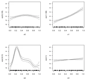
g(E(Y ))=PL= α +f1(X1)+f2(X2)+...+ ε (4) where each predictor variable, Xn, is fitted by means of a function fn( ). So, a GAM is the addition of different functions fitted to the independent variables in order to predict Y-values. Data are fitted with respect to the par-tial residuals: the residuals after removing the effect of all predictor variables (Fig. 1). Hastie and Tibshirani (1990) discuss various general scatter-plot smoothers that can be applied to the X-variable values, with the target criterion to maximize the prediction quality of the (transformed) Y-variable values. One such scatter-plot smoother is the cubic smoothing splines smoother (Wood and Augustin 2002), which generally produces a smooth generalization of the relationship between the two variables in the scatter-plot. A detailed description of how GAMs are fit to the data in relation to the algorithms used, outer and inner loop, can be found in Hastie and Tibshirani (1990). In terms of the degrees of freedom, in a parametric regres-sion one degree of freedom is lost when a single coeffi-Table 1. Limitations and advantages of linear (LM) and
general-ized regression approaches, GLM and GAM (* = linearization of predictor variables is required, = GWR is implemented in a GAM).
Non-Gaussian
distributions Link functions Non-linear fittings
LM X X √(*)
GLM √ √ √(*)
GAM √ √ √
GWR √(+) √(+) √(+)
cient is estimated. Similarly, the more complex the spline, the greater the number of degrees of freedom that are lost. Degrees of freedom can be forced by the modeller to reduce the complexity of the adjusted spline, avoiding over-fitting and obtaining response curves with an easier interpretation. There are computationally effective ways to choose the amount of smoothing as General Cross Valida-tion procedure that penalise the complexity of the model (see Wood and Augustin 2002 for a technical exposition). The GCV score is used to find the model with the highest accounted deviance using the simplest splines (e.g. GCV procedure try to maximize the trade-off between model fit and the overall smoothness. When splines are forced to a maximum of four degrees of freedom, the maximum smooth considered for each variable by GCV is four and splines are forced to present four or less complexity than four degress of freedom).
Scatter-plots in a GAM show the smoothed predictor variable values, on the X-axis, plotted against the partial residuals, on the Y-axis, and allows the modeller to under-stand the nature of the relationship between the predic-tor and the residualized dependent variable values. In this kind of plot, the fitted spline is shown with the confidence bands, 95% or 99%, and the cases appear as a rough plot at the bottom (Fig. 1). The title of the Y-axis is the name of the dependent variable with the degrees of freedom of the spline, which express the degree of complexity of each spline.
Finally, Geographically Weighted Regressions, GWR are a special case of regression approaches mainly featured by its capability to vary the regression parameters across the space. So, it could be considered as a local approach while standard regression approaches or GLMs and GAMs are global techniques, with a single set of model param-eters taken to apply uniformly in space. A GWR can be stated as:
Y= β0(ui, vi)+ xijβj(ui, vi)+
j=1 n
∑
εi (5)where there are j = 1, n explanatory variables, εi, is a ran-dom error term, the location for each observation is de-fined by the coordinates (ui, vi); β0 – βn are the parameters of the model with βj(ui, vi) a realization of the continuous function βj(u, v) at location i. Parameters are estimated weighting the contribution of an observational site in rela-tion to its spatial distance to the specific locarela-tion under consideration. The spatial weighting is achieved by means of a geographical kernel and it varies in relation to the size of the kernel: band width (see Fotheringham et al. 2002 for a specific exposition about parameter estimations, weighting functions or bandwidth selection). However, we assess here the predictive capacity of GWR but assuming non-linear fittings between response and predictor vari-ables in order to present a different insight of GWR. The
GWR is implemented in a GAM and fitted using penal-ized splines:
Y = β0(ui, vi)+ xijfj(ui, vi)+
j=1 n
∑
εi (6)where there are j = 1, n explanatory variables, εi, is a ran-dom error term, the location for each observation is de-fined by the coordinates (ui, vi); β0 (also named ε in Eq. 3 and 4) is the constant parameter of the model, with fj(ui, vi) a realization of the continuous function fj(u,v) at loca-tion I (in this case, f funcloca-tions are based here in penalised splines). Mgcv package (Wood and Augustin 2002) was also used to develop the GWR. In mgcv the smoothing parameters are basically equivalent or reciprocal to the bandwidth in a GWR.
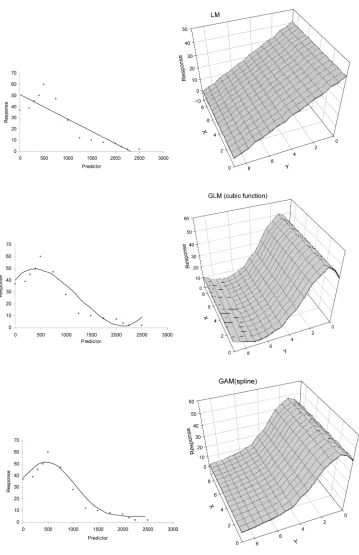
The functions adjusted by each regression approach could be applied to each pixel or other units (census grid cells, municipalities or others) for mapping the predic-tions or residuals. The selection of linear or non-linear approaches implies differences on the predictive mapping (Fig. 2), not only related to the degree of accuracy but to the assumed type of relationship between response and predictor variables.
Data, model formulation and evaluation
A terrain complexity map was obtained using a moving windows technique based on an ‘ArcInfo Macro Language’ routine over DEM map. This pitted texture index is based on perpendicular vectors and spherical variance and syn-thesizes changes in altitude, slope and aspect (Felicísimo 1994). Average values of PET and terrain complexity were extracted for the 79 UTM 100 km2 grid cells.
A land-cover map at 1:25 000, comprising 24 classes, was obtained from the Dept of Agriculture of the Regional Government of Navarra. The map was developed using orthophotos (1:25 000) and fieldwork to confirm the type of land-cover in each patch. Only the areas of three land-cover classes in each 100 km2 grid cell were selected to avoid an inadequate ratio between cases and variables. These classes are deciduous forest, heath-lands and mead-ows, and Mediterranean croplands. They were selected due to their representation of the typical land-cover of the three biogeographical environments of the study area: Atlantic, alpine and Mediterranean environments.
Landscape structure analysis was developed with ‘Geo-graphic Resources Analysis Support System (GRASS)’, and ‘r.le Programs’ (Baker and Yunming 1992). Three indeces were calculated to measure different landscape features. ‘Mean Patch Size’ represents the mean patch size of patches (polygons) in each 100 km2 grid square. The ‘Degree of Landscape Division Index’ (Jaeger 2000) shows the probability that randomly chosen sites in each 100 km2 grid square are not in the same undissected area. The ‘Shannon Diversity Index’ (Shannon and Weaver 1949) estimates land covers diversity in each 100 km2 grid square. Measures were developed using the 24 classes of the land-cover map.
Finally, one variable of each group was selected to de-velop MIX-PET, Shannon Diversity Index and the area of Mediterranean croplands were selected. Selection of the variables was developed to avoid co-linearity between variables. Thus, a previous Pearson correlation analysis us-ing the variables of TCLIM, LCAREA and LANDS was calculated in order to select variables without correlation. So, the four groups of predictor variables were developed: TCLIM, LCAREA, LANDS and MIX (Table 2).
After obtaining the four data-sets, they were used to fit each one of them against avian species richness in each of the regression approaches:
1) GLM using only linear terms was regressed against one of the mentioned groups of predictor variables. This
will be called GLM1 and represents a typical linear re-gression model, although assuming a non-gaussian dis-tribution of the response variable; 2) GLM testing linear, quadratic or cubic terms of each predictor variable. The term showing the best predictive capacity for each variable is selected to develop the final model. This will be called GLM2; 3) GAM controlling complexity of each spline to a maximum of four degrees of freedom. This will be called GAM1. Model complexity is penalised by means of GCV procedure (Wood and Augustin 2002); 4) GAM without controlled spline complexity. This will be called GAM2; 5) GWR implemented in a GAM with splines forced to a maximum of four degrees of freedom. Model complexity is penalised by GCV procedure. This will be called GWR.
The response variable is bird species richness, a special type of count data, a Poisson distribution with a log-link function, was chosen according to Crawley (1993) in each regression approach. Using a log-link function, illogical predicted values (less than 0 species) are avoided.
To assess the accuracy of the model, cross-validation was used to compare estimated with observed values. Cross-validation is an appropriate technique to evaluate models when two independent data-sets (for calibration and vali-dation) cannot be built because of the reduced number of cases (Guisan and Zimmermann 2000). This technique works by leaving out one of the cases, fitting the model to the remainder and then applying the obtained equa-tion to the previously removed case in order to calculate its predicted value. This procedure is repeated for each case in the data-set. The values predicted from cross-validation were used to calculate an error estimator (Willmott 1982) Willmott’s D:
D=1−
Pi −Oi
(
)
2i=1 N
∑
Pi'
+ Oi'
(
)
2i=1 N
∑
(7)
where N = number of observations, O = Observed val-ue, O= mean of observed values, P = predicted value, i = counter for individual observed and predicted values,
Pi'
=Pi−O and Oi'
=Oi−O. Willmott’s D varies from 0 to 1 (1 means a perfect prediction). Willmott’s D was calculated for the twenty models. The average of the Willmott’s D values was obtained for each regression
Table 2. The four groups of predictor variables: climate and topography (TCLIM), area of main land-covers (LCAREA), landscape structure variables (LANDS) and a mixture of variables belonging to the first three groups.
TCLIM LCAREA LANDS MIX
PET Area of deciduous forest Mean Patch Size PET
technique (GLM1, GLM2, GAM1, GAM2 and GWR) to provide a synthesis of their predictive accuracy.
Finally, some plots are shown to comment on the spe-cific problems of GAMs in relation to the interpretation of complex splines.
Data analyses were developed using the R (Ellner 2001, <www.r-project.org>) and mgcv packages (Wood and Au-gustin 2002); both are non-commercial, open source soft-ware. Also, another package exists in R to calculate GAM in spatial frameworks: Generalised Regression Analysis and Spatial Predictions (GRASP, Lehmann et al. 2002b). R software implements packages to connect statistical analysis with some GIS applications such as GRASS or Arc View.
Results
Model evaluation
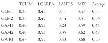
GWR with splines show highest predictive values (Will-mott’s D: 0.47) when the five multi-variable regression ap-proaches are regressed against TCLIM predictor variables (Table 3), followed by GAM1 and GAM2. Both methods show a value of 0.40 for the error estimator D, since fitted splines have the same degree of complexity (1.23 estimated degrees of freedom: EDF). This is due to the existence of linear or quasi-linear relationships between response and predictor variables. Similarly, GLM1 and GLM2 show the same D-value, 0.35, because linear terms were the best predictors of response variable when linear, quadratic and cubic terms were tested for GLM2. GWR is the more ac-curate approach when regressed against LANDS predic-tor variables (0.43), followed by GAM2 (0.35), GAM1 (0.23), GLM2 (0.14) and finally GLM1, which shows a D-value of 0.11. GWR is the more accurate model when LCAREA variables are used (0.55), followed by GAM2 and GAM1 (0.53), GLM2 (0.45), and GLM1, which shows only 0.35 for the error estimator D. Again, GWR is the more accurate model when MIX-predictor variables are used, 0.68, followed by GAM2 (0.62), GAM1 (0.59).
Under these conditions, GLM2 and GLM1 present D-values of 0.51 and 0.47, respectively.
An average of the D-values for each regression ap-proach was obtained to summarize the results. GWR showed the highest average D-value (0.53) followed by GAM2 (GAM without controlling spline complexity), GAM1, GLM2 and GLM1 (Table 3). Thus, GWR ex-hibits a 20% higher predictive accuracy than the worst approach, GLM1, whilst GAM2 exhibits a 13% GAM2 exhibits a 9% improvement over GLM1 (50% is equal to an improvement of 0.5 in Willmott’D). Finally, GLM2 only shows a 1% improvement over GLM1. Also, GWR is the most accurate model in all the groups of variables (TCLIM, LANDS, LCAREA, MIX), followed by GAM2 and GAM1 (Table 3).
Plot interpretation
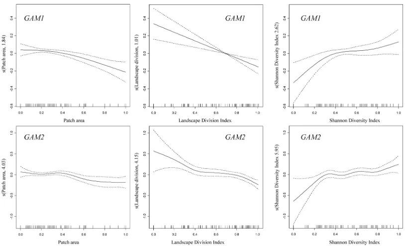
Scatter-plots of the relationships between LANDS vari-ables and bird species richness are shown to highlight the specific problems of GAMs in relation to spline complex-ity. The plots obtained using GAM1 and GAM2 to model species richness using LANDS variables show a similar re-lationship between species richness and predictor variables (Fig. 3). An increment in land-cover diversity is correlated with an increment in avian species richness, whilst an in-crease in land-cover fragmentation implies a reduction of species richness. Finally, bigger patches imply lower species richness. However, visual inspection of the plots indicates that splines fitted without controlling their degrees of free-dom are more complex, as stated in Table 4; the implica-tions of this observation will be discussed below.
Discussion and conclusions
This work has attempted to present a synthesis of gen-eralised regression models, GLM and GAM (including a GWR approach), and to assess the improvement of predic-tive accuracy of these emerging tools in comparison with the traditional lineal regressions. As mentioned in the regression descriptions, generalised models allow model-lers to choose from different distributions of the response variable (normal, gamma, Poisson and bi-nomial for di-chotomous response variables) and different link func-tions (identity, inverse, log, power or log-it). Also, GAM supports the fitting of non-linear relationships, improving the levels of explained deviance but also providing a more rational explanation of the nature of some relationships. Non-linear relationships are not infrequent in nature and spatial models need to take them into consideration (Jongman et al. 1995). Linear approaches do not fit this relationship adequately and the predictive maps obtained do not make much sense, as stated in Fig. 2. In addition, GAMs allow time consumption to be reduced, because Table 3. Willmott’s D-values for each model using the different
regression approaches. Average of D-values was obtained for each type of regression.
TCLIM LCAREA LANDS MIX Average
GLM1 0.35 0.45 0.11 0.47 0.35
GLM2 0.35 0.45 0.14 0.51 0.36
GAM1 0.40 0.53 0.23 0.59 0.44
GAM2 0.40 0.53 0.35 0.62 0.48
non-linear curves (splines) are automatically adjusted and no time needs to be spent on testing linear, quadratic or cubic terms, as is the case in GLM. On the other hand, GWRs offer local fitting of regression parameters and its implementation in a GAM framework seems to be a pow-erful tool for spatial predictions.
Generalised Additive Models, including a GWR ap-proach, tested here in a GAM framework, offer the highest levels of predictive accuracy. The improvement in predic-tive accuracy obtained using GAMs in relation to con-ventional regressions, although with some variations, has been tested by other authors in ecological studies compar-ing GAM with other approaches (Bishop and McBratney 2001, Hirzel et al. 2001, Pearce and Ferrier 2002, Rob-ertson et al. 2003, Thuiller 2003, Brotons et al. 2004). In hydrological research, studies using different predictive methods (Elder et al. 1998, Chang and Li 2000), includ-ing regression trees, have shown predictive levels of simi-lar or lower accuracy than GAM, mainly when validation
techniques such as cross-validation are used in addition to r2 or explained deviance (López-Moreno and Nogués-Bravo 2005). Also, methods such as regression trees and Artificial Neural Networks (ANN) lose environmental in-terpretability, because they do not allow the observation of response curve shapes (Lehmann et al. 2002a). In a paper focused on soil property mapping (Bishop and McBrat-ney 2001), GAMs represented the second best approach behind kriging with external drift. In a similar way, Foody (2003) also underlined the improvement reached in pre-dictive accuracy using GWR in comparison with ordinary least (OLS) regression analysis. Naturally our results are contingent on the particular data-set although they are similar to other works cited in this paragraph.
In relation to the effect of spline complexity on predic-tive accuracy, GAM2 offers an improvement on GAM1, GAM with splines complexity controlled to four degrees of freedom, of 7.2% in the average values of D. How-ever, this improvement is supported by an increment in the degrees of freedom used: 15.1 EDF in all models of GAM1 against 24 EDF in all models of GAM2. This situation is highlighted when GAM approaches are evalu-ated against LANDS variables, since 5.45 EDF are lost by GAM1, whilst GAM2 uses 14.13 EDF. This implies that the robustness of GAM1 is higher than that of GAM2 and, consequently, the prediction improvement (7.2%) should not justify the use of splines without complexity penalisation. Consequently, in agreement with Wood and Augustin (2002), controlling splines complexity to a maxi-Figure 3. Estimated terms describing the dependence of avian species richness on LANDS variables (landscape variables). Estimates (solid) and 95% confidence intervals (dashed). Splines penalised to a maximum of four degrees of freedom (GAM1) are less com-plex.
Table 4. Estimated degrees of freedom (EDF) used by GAM1, GAM2 and GWR approaches.
TCLIM LCAREA LANDS MIX Sum
GAM1 2 2.98 5.462 4.7 15.14
GAM2 2 3.21 14.132 4.7 24.04
mum number of degrees of freedom, such as four, could be considered as an adequate compromise between predictive accuracy, statistical robustness and curve interpretation. Usually, the more complex the model is, the better the fit is. However, there is not reason to inflate the complex-ity of models for accounting more deviance since a slight improvement of predictive accuracy could be based in an important reduction of model parsimony.
Statistical models for spatial predictions attempt to achieve two main objectives: to obtain a reliable estima-tion of the object under study in unsampled areas or in future scenarios and to evaluate theories about the factors driving the spatial distribution of the object under study. Anyway, correlation does not imply causation and obtain-ing inference from statistical model is a debatable ques-tion (MacNally 2000, 2002). So, advanced statistical ap-proaches, like those presented here, could be considered as efficient predictive techniques but their role as explanatory tools could be affected, for example, by spatial auto-corre-lation (Legendre and Legendre 1998, Fotheringham and Brunsdon 2004) or co-linearity between variables.
In conclusion, the necessity of developing support deci-sion tools implemented in spatial frameworks using GIS, implies the development of powerful and flexible method-ologies. Thus, accurate predictive tools oriented towards modelling spatial patterns of different features should be used in order to maximize the accuracy of models and the assessment of different techniques and routines should be considered. The application of Generalised Additive Mod-els, an emerging predictive tool in ecology and biomedi-cal sciences over the last years, but scarcely used in other research fields, could improve the results obtained. The improvement on predictive accuracy obtained by GAMs is mainly based on non-linear fits. Finally, Geographically Weighted Regressions using flexible splines add a surplus of accuracy in predictive models related to the local varia-tion of regression parameters.
References
Anderson, R. P. et al. 2003. Evaluating predictive models of spe-cies distributions: criteria for selecting optimal models. – Ecol. Modell. 162: 211–232.
Araújo, M. B. et al. 2008. Exposure of European biodiversity to changes in human-induced pressures. – Environ. Sci. Policy 11: 38–45.
Austin, M. P. 2002. Spatial prediction of species distribution: an interface between ecological theory and statistical modelling. – Ecol. Modell. 157: 101–118.
Baker, L. W. and Yunming, C. 1992. The r.le programs for multiscale analysis of landscape structure using the GRASS geographical information system. – Landscape Ecol. 7: 291–302.
Barry, S. C. and Welsh, A. H. 2002. Generalized additive mod-elling and zero inflated count data. – Ecol. Modell. 157: 179–188.
Beckmann, B. and Buishand, T. 2002. Statistical downscaling relationships for precipitation in the Netherlands and north Germany. – Int. J. Climatol. 22: 15–32.
Bishop, T. F. A. and McBratney, A. D. 2001. A comparison of prediction methods for the creation of field-extent soil prop-erty maps. – Geoderma 103: 149–160.
Brotons, L. et al. 2004. Presence–absence versus presence-only modelling methods for predicting bird habitat suitability. – Ecography 27: 437–448.
Brown, J. H. et al. 2002. The fractal nature: power laws, ecologi-cal complexity and biodiversity. – Philos. Trans. R. Soc. B 357: 619–626.
Brunsdon, C. et al. 1996. Geographically weighted regression: a method for exploring spatial non-stationarity. – Geogr. Anal. 28: 281–298.
Brunsdon, C. et al. 2001. Spatial variations in the average rain-fall-altitude relationship in Great Britain: an approach using geographically weighted regression. – Int. J. Climatol. 21: 455–466.
Carey, P. D. 1996. A cellular automaton for predicting the distri-bution of species in a changed climate. – Global Ecol. Bio-geogr. 5: 217–226.
Cawsey, E. M. et al. 2002. Regional vegetation mapping in Aus-tralia: a case study in the practical use of statistical modelling. – Biodiv. Conserv. 11: 2239–2274.
Chang, K. and Li, Z. 2000. Modelling snow accumulation with a geographic information system. – Int. J. Geogr. Inf. Sci. 14: 693–707.
Crawley, M. J. 1993. GLIM for ecologists. – Blackwell. De’ath, G. and Fabricius, K. 2000. Classification and regression
trees: a powerful yet simple technique for ecological data analysis. – Ecology 81: 3178–3192.
Elder, K. et al. 1998. Estimating the spatial distribution of snow water equivalence in a montane watershed. – Hydrol. Proc. 12: 1793–1808.
Ellner, S. P. 2001. Review of R, ver. 1.1.1. – Bull. Ecol. Soc. Am. 82: 127–128.
Felicisimo, A. M. 1994. MDT: introducción y aplicaciones en las ciencias ambientales. – Pentalfa, Oviedo.
Foody, G. M. 2003. Geographical weighting as a further refine-ment to regression modelling: an example focused on the NDVI-rainfall relationship. – Remote Sens. Environ. 88: 283–293.
Foody, G. M. 2004. Spatial non-stationary and scale-dependen-cy in the relationships between species rihcness and environ-mental determinants for the sub-Saharan endemic avifauna. – Global Ecol. Biogeogr. 13: 315–320.
Fotheringham, S. A. and Brunsdon, C. 2004. Some thoughts on inference in the analysis of spatial data. – Int. J. Geogr. Inf. Sci. 18: 447–457.
Fotheringham, A. S. et al. 2002. Geographically weighted regres-sion: the analysis of spatially varying relationships. – Wiley. Frencht, J. L. and Wand, M. P. 2004. Generalized additive
mod-els for cancer mapping with incomplete covariates. – Biosta-tistics 5: 177–191.
Goodchild, M. F. 2001. Models of scale and scales of modelling. – In: Tate, N. J. and Atkinson, P. M. (eds), Modelling scale in geographical information science. Wiley, pp. 3–11. Guisan, A. and Zimmermann, N. E. 2000. Predictive habitat
Guisan, A. et al. 2002. Generalized linear and generalized ad-ditive models in studies of species distributions: setting the scene. – Ecol. Modell. 157: 89–100.
Haines-Young, R. et al. 1993. Landscape ecology and GIS. – Taylor and Francis.
Hastie, T. and Tibshirani, R. 1990. Generalized additive models. – Chapman and Hall.
Heargraves, G. L. 1985. Defining and using reference evapotran-spiration. – J. Irrig. Drain. E-Asce. 120: 1132–1139. Hirzel, A. H. et al. 2001. Assessing habitat-suitability models
with a virtual species. – Ecol. Modell. 145: 112–121. Jaeger, J. A. G. 2000. Landscape division, splitting index, and
effective mesh size: new measures of landscape fragmenta-tion. – Landscape Ecol. 15: 115–130.
Janet, F. 1998. Predicting the distribution of shrub species in southern California from climate and terrain-derived vari-ables. – J. Veg. Sci. 9: 733–748.
Johnston, R. J. et al. 2002. Geographies of global change: remap-ping the world. – Blackwell.
Jongman, R. H. G. et al. 1995. Data analysis in community and landscape ecology. – Cambridge Univ. Press.
Legendre, P. and Legendre, L. 1998. Numerical ecology. – El-sevier.
Lehmann, A. et al. 2002a. Regression models for spatial predic-tion: their role for biodiversity and conservation. – Biodiv. Conserv. 11: 2085–2092.
Lehmann, A. et al. 2002b. GRASP: generalized regression analy-sis and spatial prediction. – Ecol. Modell. 157: 189–207. López-Moreno, J. I. and Nogués-Bravo, D. 2005. Mapping the
spatial distribution of snow pack in the Spanish central Pyr-enees. – Hydrol. Proc. 19: 3167–3176.
López-Moreno, J. I. et al. 2006. Change of topographic control on the extent of cirque glaciers since the Little Ice Age. – Geophys. Res. Lett. 33: L24505.
MacNally, R. 2000. Regression and model building in conserva-tion biology, biogeography and ecology: the distincconserva-tion be-tween – and reconciliation – of ‘predictive’ and ‘explanatory’ models. – Biodiv. Conserv. 9: 655–671.
MacNally, R. 2002. Multiple regression and inference in ecol-ogy and conservation biolecol-ogy: further comments on identi-fying important predictor variables. – Biodiv. Conserv. 11: 1397–1401.
Maidment, D. and Djokic, D. 2000. Hydrologic and hydraulic modelling support with geographic information systems. – ESRI Press.
Manel, S. et al. 1999. Comparing discriminant analysis, neural networks and logistic regression for predicting species dis-tribution: a case study with Himalayan river bird. – Ecol. Modell. 120: 337–347.
McCullagh, P. and Nelder, J. A. 1989. Generalized linear models. – Chapman and Hall.
Nogués, D. and Martínez-Rica, J. P. 2004. Factors controlling the spatial species richness pattern of four groups of ter-restrial vertebrates in an area between two different bio-geographic regions in northern Spain. – J. Biogeogr. 31: 629–640.
Nogués-Bravo, D. and Aguirre, A. 2006. Modelling the spatial distribution and habitat selection of Dupont’s Lark Cher-shopilus duponti in northern Spain. – Ardeola 53: 55–68. Nogués-Bravo, D. and Araújo, M. B. 2006. Species richness,
area and climate correlates. – Global Ecol. Biogeogr. 15: 452–460.
Osborne, P. E. and Suarez-Seoane, A. 2002. Should data be parti-tioned spatially before building large-scale distribution mod-els? – Ecol. Modell. 157: 249–259.
Pearce, J. and Ferrier, S. 2002. An evaluation of alternative algo-rithms for fitting species distribution models using logistic regression. – Ecol. Modell. 128: 127–147.
Peters, R. H. 1991. A critique for ecology. – Cambridge Univ. Press.
Rigol, J. P. et al. 2001. Artificial neural networks as a tool for spatial interpolation. – Int. J. Geogr. Inf. Sci. 15: 323–343. Robertson, M. P. et al. 2003. Comparing models for predicting
species potential distributions: a case study using correlative and mechanistic predictive modelling techniques. – Ecol. Modell. 164: 153–167.
Schwartz, J. 1999. Air pollution and hospital admissions for heart disease in eight US counties. – Epidemiology 10: 17–22. Shannon, C. E. and Weaver, W. 1949. The mathematical theory
of communication. – Univ. of Illinois Press, Urbana. Stassopoulou, A. 1998. Application of a Bayesian network in a
GIS based decision making system. – Int. J. Geogr. Inf. Sci. 12: 23–46.
Stockwell, D. and Peters, D. 1998. The GARP modelling sys-tem: problems and solutions to automated spatial predic-tion. – Int. J. Geogr. Inf. Sci. 13: 143–158.
ter Braak, C. J. F. 1988. CANOCO: an extension of DECO-RANA to analyze species relationships. – Vegetatio 75: 159–160.
Thuiller, W. 2003. BIOMOD – optimizing predictions of spe-cies distributions and projecting potential future shifts under global change. – Global Change Biol. 9: 1353–1362. White, D. and Sifneos, J. 2002. Regression tree cartography. – J.
Comput. Graph. 11: 600–614.
Whittaker, R. J. et al. 2007. Geographic gradients of species richness: a test of the water-energy conjecture of Hawkins et al. (2003) using European data for five taxa. – Global Ecol. Biogeogr. 16: 76–84.
Willmott, C. 1982. Some comments on the evaluation of model performance. – Am. Meteorol. Soc. 63: 1309–1313. Wood, S. N. and Augustin, N. H. 2002. GAMs with intergrated
model selection using penalized regression spline applica-tions to environmental modelling. – Ecol. Modell. 157: 157–177.
WMO 1967. A note on climatological normals, WMO no. 208. T. N. no. 84. – World Meterological Organization, Geneva, Switzerland.
Yee, T. W. and Mackenzie, M. 2002. Vector generalized additive models in plant ecology. – Ecol. Modell. 157: 151–156. Zaniewski, A. E. et al. 2002. Predicting species spatial