CAAS: an atmospheric correction algorithm for the remote sensing of complex waters

www.ann-geophys.net/30/203/2012/ doi:10.5194/angeo-30-203-2012

© Author(s) 2012. CC Attribution 3.0 License.

Annales

Geophysicae

CAAS: an atmospheric correction algorithm for the remote sensing

of complex waters

P. Shanmugam

Ocean optics and Imaging Laboratory, Department of Ocean Engineering, Indian Institute of Technology Madras, Chennai – 600036, India

Correspondence to: P. Shanmugam ([email protected])

Received: 31 May 2011 – Revised: 23 December 2011 – Accepted: 10 January 2012 – Published: 18 January 2012

Abstract. The current SeaDAS atmospheric correction al-gorithm relies on the computation of optical properties of aerosols based on radiative transfer combined with a near-infrared (NIR) correction scheme (originally with assump-tions of zero water-leaving radiance for the NIR bands) and several ancillary parameters to remove atmospheric effects in remote sensing of ocean colour. The failure of this algo-rithm over complex waters has been reported by many recent investigations, and can be attributed to the inadequate NIR correction and constraints for deriving aerosol optical prop-erties whose characteristics are the most difficult to evaluate because they vary rapidly with time and space. The possi-bility that the aerosol and sun glint contributions can be de-rived in the whole spectrum of ocean colour solely from a knowledge of the total and Rayleigh-corrected radiances is developed in detail within the framework of a Complex wa-ter Atmospheric correction Algorithm Scheme (CAAS) that makes no use of ancillary parameters. The performance of the CAAS algorithm is demonstrated for MODIS/Aqua im-ageries of optically complex waters and yields physically re-alistic water-leaving radiance spectra that are not possible with the SeaDAS algorithm. A preliminary comparison with in-situ data for several regional waters (moderately complex to clear waters) shows encouraging results, with absolute er-rors of the CAAS algorithm closer to those of the SeaDAS algorithm. The impact of the atmospheric correction was also examined on chlorophyll retrievals with a Case 2 wa-ter bio-optical algorithm, and it was found that the CAAS algorithm outperformed the SeaDAS algorithm in terms of producing accurate pigment estimates and recovering areas previously flagged out by the later algorithm. These findings suggest that the CAAS algorithm can be used for applica-tions focussing in quantitative assessments of the biological and biogeochemical properties in complex waters, and can easily be extended to other sensors such as OCM-2, MERIS and GOCI.

Keywords. History of geophysics (Atmospheric sciences; Ocean sciences) – Radio science (Remote sensing)

1 Introduction

Use of the near synoptic and global data provided by satellite sensors such as MODIS-Aqua (Moderate Resolution ing Spectroradiometer), MERIS (MEdium Resolution Imag-ing Spectrometer) and OCM2 (Ocean Colour Monitor 2) that build upon the CZCS (Coastal Zone Colour Scanner) and SeaWiFS (Sea-viewing Wide Field-of-view Sensor) heritage has become an essential component of the coastal oceano-graphic research and monitoring. These instruments measure the spectrum of sunlight reflected from the ocean-atmosphere system at several visible and near-infrared (NIR) wavebands. The major portion of these signals is from the contribution of scattering by molecules and particles (aerosols) in the at-mosphere (∼80–90 %). The process of removing the atmo-spherically scattered signal in order to retrieve the desired ocean colour signal (i.e. water-leaving radianceLw)is

re-ferred to as atmospheric correction (Gordon, 1997). Since simultaneous measurements of atmospheric optical proper-ties are not available, the atmospheric correction algorithm developed for SeaWiFS and MODIS (also referred to as SeaDAS atmospheric correction algorithm) assumes negli-gibleLw in the bands centred at 765 and 865 nm (748 and

869 nm in case of MODIS) in order to derive aerosol op-tical properties and extrapolate these into the visible spec-trum (Gordon and Wang, 1994). This procedure is termed as the dark-pixel atmospheric correction scheme which has been widely used for clear ocean waters, where satisfactory results have been found with uncertainties<5 % inLw and

down for optically more complex waters that are classified in the context of the present study into four types: (1) wa-ters in the presence of intense aerosols (absorbing and non-absorbing), (2) waters with dense phytoplankton blooms, (3) waters with high particulate (suspended matter-SS) and dissolved substances (CDOM), and (4) waters with combina-tion of the above types and nature (all these categories belong to Case 2 waters). Though these regions are of great interest to the scientific community, resource managers and climatol-ogists, due to errors in atmospheric correction, possibilities of determination of full spectra of water-leaving radiance are very limited andLw(412)<0.2 mW cm−2µm−1sr−1are

of-ten excluded to minimize the impacts from atmospheric over-correction in causing negative or significantly reduced water-leaving radiance (Siegel et al., 2002). This eventually leads to a tremendous loss of information for ocean colour work (Doerffer et al., 2008).

To overcome the black pixel assumption that progressively degrades Lw signals with increasing suspended load (SS)

and algal blooms in nearshore waters, a number of authors have proposed modifications to account for non-negligible Lw(λNIR1 andλNIR2)within the framework of the SeaDAS

atmospheric correction algorithm (Arnone et al., 1998; Rud-dick et al., 2000; Siegel et al., 2000; Hu et al., 2000; Stumpf et al., 2003; Lavender et al., 2005). Relaxing the black pixel assumption through these modifications in the correction of satellite ocean colour data has shown significant improve-ments in theLw(λ) and Chl-a retrievals under normal

cir-cumstances (i.e. weak blooms/plumes and weak aerosol con-ditions). More recently, Wang and Shi (2007) recommended using shortwave infrared (SWIR, 1240 and 2130 nm) bands for atmospheric correction of MODIS-Aqua data in mod-erately turbid regions. However, a decade-long time-series of nLw(λ) from MODIS-Aqua in complex waters

(Chesa-peake Bay) derived using NIR and SWIR bands for atmo-spheric correction demonstrates that low signal-to-noise ra-tios (SNR) for the SWIR bands of MODIS-Aqua added noise errors to the derived radiances, which produced broad, flat frequency distributions of nLw(λ)relative to those produced

using the NIR bands (Werdell et al., 2010). They also noted that the SWIR approach produced an increased number of negative nLw(λ) and decreased sample size relative to the

NIR approach. Their results imply that poor SNR values for the MODIS-Aqua SWIR bands remain the primary defi-ciency of the SWIR-based atmospheric correction approach. On the other hand, applying NIR and SWIR bands for at-mospheric correction of MODIS-Aqua data in dense bloom waters gives nearly the same results with negatively biased Lw(412) signals for the bloomed area (Amin et al., 2009).

Many factors, such as (1) the breakdown of the black-pixel assumption in the NIR/SWIR spectral region due to algal blooms or other particles in the coastal ocean, and (2) insuf-ficient or inadequate aerosol models adopted for atmospheric correction, influence the accuracy of atmospheric correction algorithms and thereby of ocean colour retrievals (Yan et al.,

2002). The quality of such retrievals with such algorithms becomes increasingly questionable in all four situations men-tioned earlier. Additional problems and complications are encountered when optical properties of atmospheric aerosol in the considered region demonstrate very strong diversity and often do not satisfy the assumptions and invalidate a NIR approach with the SeaDAS algorithm. In particular, due to absorption effects, aerosol radiance of the desert dust is weaker at the shorter wavelengths than any of those mod-els, and cannot be accounted for adequately (Gordon, 1997). Besides, influence of strongly absorbing aerosols shows a significant dependence on their vertical distribution. This problem has been recently considered in few studies (e.g. Moulin et al., 2001; Nobileau and Antoine, 2005). The gen-eral approach is based on the coupled modeling of the optical properties of sea water and atmospheric aerosol. Such ap-proaches are applicable for Case 1 ocean waters only, but the complex waters do not belong to Case 1 type. An alternate method has been developed for deriving aerosol properties solely from the sensor-measured signal for atmospheric cor-rection of SeaWiFS imagery in the presence of strongly ab-sorbing aerosols (Shanmugam and Ahn, 2007a). While this method shows a considerable promise in retrieving reliable Lw(λ) values under these conditions, it requires additional

data for its operational utility. Thus, it is necessary to look for a different algorithm that relies solely on the total and Rayleigh-corrected radiances to derive atmospheric proper-ties and oceanic signals without involving many assump-tions and ancillary data. The algorithm should be sensor-independent so that it can be applied to any (current and fu-ture) sensors to retrieve an unbiased estimate ofLw(λ)

val-ues. Merging these different sources of information into a unique dataset not only increases data availability for a cer-tain complex area, but also increases the quality of informa-tion retrieved from the ocean (M´elin et al., 2007). Such data are highly desired by the scientific community for studying optical and biological properties of marine waters, address-ing marine environmental issues, and investigataddress-ing a variety of topics including marine primary productivity, ecosystem dynamics, sedimentation and pollution.

2 Mathematical description of the algorithm (CAAS)

The total signal (Lt)received by a sensor at the top of the

at-mosphere (TOA) in a spectral band cantered at a wavelength λi, is conveniently described in terms of radiance and decom-posed into the following components:

Lt(λi)=Lp(λi)+T Lsg(λi)+t Lwc(λi)+t Lw(λi) (1) whereLp(λi) is the path radiance resulting from scattering in the atmosphere and from specular reflection of atmospheri-cally scattered light (skylight) from the sea surface,Lsg(λi) is the radiance of direct sun glint from the sea surface,Lwc(λi) is the radiance of whitecaps at the sea surface, Lw(λi) is the desired water-leaving radiance, andT (λi)andt (λi)are the respective direct and diffuse transmittances of the at-mospheric column. The whitecap contribution Lwc(λi) in ocean colour data can be estimated by using a previously established reflectance model with the input of sea surface wind speed (Koepke, 1984). However, Gordon and Wang (1994) noted that the whitecap reflectance model used in the SeaDAS algorithm produces unacceptable errors (overesti-mation of the whitecap contribution) when the sea surface wind speed is greater than 8 m s−1_{. This leads to the}

un-derestimation of water-leaving radiances in those regions. To avoid such a miscalculation, the whitecap contribution Lwc(λi) is ignored for brevity. Then, Eq. (1) reduces to Lt(λi)=Lp(λi)+T (λi)Lsg(λi)+t (λi)Lw(λi) (2) whereLp(λi)=Lr(λi)+La(λi)+Lcpl(λi).

The path radiance is further decomposed into the follow-ing components, assumfollow-ing that radiances due to aerosol or molecular scattering are separable:Lr(λi), the radiances due

to scattering by the air molecules (Rayleigh scattering in the absence of aerosols);La(λi), the radiances due to scattering

by aerosols (in the absence of air molecules); andLcpl(λi), the radiances (coupled term) due to multiple interaction be-tween molecules and aerosols. It should be noted thatLr(λi) at all visible and NIR wavelengths depends on the atmo-spheric molecular composition, the sun and viewing geom-etry, and, weakly, on sea-surface roughness (Gordon et al., 1988; Gordon and Wang, 1992). Given the surface atmo-spheric pressure (to determine the value ofτr)and surface

wind speed (to determine the roughness of the sea surface), Lr(λi) can be computed accurately without use of the re-motely sensed radiometric data (Gordon et al., 1988; Gordon and Wang, 1992). Subtraction ofLr(λi)fromLt(λi)gives

the Rayleigh-corrected (Lrc(λi))radiance, which is defined

as

Lrc(λi)=Lt(λi)−Lr(λi) (3)

=La(λi)+Lcpl(λi)+T (λi)Lsg(λi)+t (λi)Lw(λi)

Aerosol radiance cannot be obtained without a priori knowl-edge in a similar way, because aerosol optical properties can

vary substantially over short time and space scales. Accu-rate estimation of La(λi) andLcpl(λi) requires in-situ field

measurements of aerosol type, optical thickness, air pressure, wind, water vapour, etc., at the time of each image acquisi-tion. These measurements are frequently unavailable or are of questionable quality which makes routine and accurate at-mospheric correction of satellite images with radiative trans-fer models difficult (Song et al., 2000). Furthermore, scat-tering and absorption by aerosols are difficult to characterize due to their variation in time and space (Gordon and Wang, 1994), thus constituting the most severe limitation to the atmosphere correction of satellite data (Coppin and Bauer, 1994). Thus, the SeaDAS assumes zero ρw for λNIR1 and

λNIR2 to derive the aerosol typeε=ρas(λNIR1)/ρas(λNIR2)

(more recently assumption of zeroρwat NIR bands has been

replaced with a NIR correction scheme, Werdell et al., 2010), uses this to select the most appropriate aerosol model from a family of N aerosol models for different solar and view-ing geometries, and on the basis of the selected model de-rives aerosol information from NIR into the visible. Sub-tracting this from the total yields the full set of water-leaving reflectances ρ(λ), which include implicitly zero values for ρw(λNIR1)andρw(λNIR2)and improbable large negative

val-ues forρw(λ412−λ443)in complex waters. This problem is

more severe in waters with algal blooms (e.g. Arabian Sea), where large negative values are also produced at other vis-ible bands. To avoid a number of assumptions and further refinements needed for an extension of the SeaDAS algo-rithm to such waters, aerosol radiances at near-infrared bands (La(λNIR1)andLa(λNIR2)) are iteratively derived from the

spectral information ofLrc(λi)through the following

spec-tral models:

La(λNIR1)=Lrc(λNIR1)−Lac(λNIR1)

La(λNIR2)=Lrc(λNIR2)−Lac(λNIR2)

(4) where aerosol corrected radiances (Lac)for the NIR bands

that are derived as follows: Lac(λNIR1)=

Lrc(λNIR2)

Lrc(λNIR1)2

× {[[Lrc(λNIR1)−Lrc(λNIR2)] ×Lrc(λNIR1)]−

Lrc(λNIR2)

π × [Lrc(λ412)−Lrc(λNIR2)]

×[Lrc(λNIR1)−Lrc(λNIR2)]]} (5)

Lac(λNIR2)=

Lac(λNIR1)

π (6)

Because the reliable estimation ofLa(λi)is necessary for the visible and NIR bands, La(λNIR1)andLa(λNIR2)are used

in the second iteration to obtain new aerosol radiances at all wavelengths through Eqs. (7) and (8).

La(λi)=Lrc(λi)−Lac(λi) (7)

Lac(λi)=

La(λNIR2)

La(λNIR1)2

×La(λNIR1)]−

hL_a(λ_NIR2)

π × [Lrc(λ412)−La(λNIR2)]

×[La(λNIR1)−La(λNIR2)] io

(8) The estimates of La(λi) are reasonably comparable with

those of the SeaDAS algorithm for open ocean waters where aerosols occur locally. However, for coastal watersLa(λi)

derived from CAAS differ with those of the SeaDAS algo-rithm because these regions usually have both Case 2 wa-ters in which theρwat the two NIR bands are discarded or

the estimatedρwin these bands are insufficient to deal with

bloom/turbid waters and strongly absorbing aerosols (Shan-mugam and Ahn, 2007a, b).

One of the major confounding factors limiting the quality and accuracy of ocean colour data is sun glint, the specular reflection of directly transmitted sunlight from the upper side of the air-water interface (Doerffer et al., 2008; Kay et al., 2009). The sun glint correction is an extension of the atmo-spheric correction. Data of sensors such as MODIS, MERIS and OCM2, which have no capability to tilt the sensor in for-ward or backfor-ward direction to avoid or reduce the influence of sun glint, are contaminated with glint patterns, which may often cover more than half of the image. Without an accurate correction these data are lost for retrieving optical properties of the water or the concentrations of substances (Doerffer et al., 2008). Its distribution depends on the solar and obser-vation angles and the roughness of the sea (wind dependent wave slopes), and can be defined as follows:

nLsg(λi)= Lsg(λi)

T (λi) (9)

where nLsg(λi) is the normalized sun glint radiance and T (λi)is assumed unity. Though methods based on the Cox and Munk model are used with most of the ocean colour in-struments now in operation they do have limitations. The wind data may not have sufficient resolution to capture the effects of local winds, and the Cox and Munk model does not include the effects of atmospheric stability, wind age or swell (Hwang and Shemdin, 1988). Furthermore, aerosol values are particularly hard to separate from the glint signal, since the “effect” that increases with aerosol load is not the glint itself but the error due to the single scattering approx-imation (Kay et al., 2009). To estimate the sun glint radi-ance (Lsg), the model involves measurements of La(λ412),

Lac(λ412), Lt(λ412), and Lrc(λ412) (assuming glint

infor-mation contained in all these products) to calculateLsg at

412 nm with the following criteria:

Lsg(λ412)=

Lrc(λ412)

Lt(λ412)

× [La(λ412)−Lac(λ412)] (10)

IfLsg<0

Lsgc(λi)=Lac(λi)

wherei=412∼551. IfLsg>0

Lsgc(λi)=Lac(λi)−Lsg(λi)

wherei=412∼551.

The relative amount of sun glintLsg(λi)can be obtained

by an exponential function withLsg(λ412)as an input;

Lsg(λi)=Lsg(λ412)×exp(λi/λ869) (11)

Our analysis shows that the slightly higher values of Lsg(λ412)from Eq. (11) are adequate for its correction at

longer wavelengths (λ667−λ869 with similar criteria). The

sun glint corrected radianceLsgc(λi)is as follows:

Lsgc(λi)=Lt(λi)−Lr(λi)−La(λi)−T (λi)Lsg(λi)

=Lcpl(λi)+t (λi)Lw(λi) (12) The water-leaving radiancet (λi)Lw(λi)exiting the TOA can

be retrieved if the coupled aerosol termLcpl(λi)is known. However, this component is very complex and its estima-tion is critical because it often deteriorates the accuracy of Lw(λi)(Gordon and Voss, 1999). Removal ofLcpl(λi)can be achieved through a spectral model that takes the following form of equation to provide estimates oft (λi)Lw(λi): t (λi)Lw(λi)=

(υ(λi))(λi/λNIR2)υ0(λi)

λ₄₁₂

λNIR2

−[1ε(λi,λNIR2)×La(λNIR2)] (13)

The(υ(λi))(λi/λNIR2) andυ0(λi)are obtained independently with two models that behave quite differently according to: υ(λi)=Lsgc(λi)−

La(λi)−Lrc(λi) Lrc(λi)−Lsgc(λi)

(14)

υ0(λi)=Lsgc(λi)−

−

_L

a(λi)−La(λNIR2)

Lrc(λi)−Lsgc(λi)

(15)

The above corrections are necessary because the aerosols are many types (strongly absorbing and non-absorbing) and may consist of a multi-component mixture of particles with dif-ferent chemical compositions (that change with differing hu-midity and altitude) and affinities to water (Yan et al., 2003). It has been noted that under these circumstances, models with the SeaDAS algorithm remove too muchLcpl(λi)from

sensor-observed radiance which eventually leads to a non-negligible error in the retrieval of ocean colour (Li et al., 2003). The above spectral models (Eqs. 14 and 15) overcome a number of shortcomings, thereby deriving and effectively removing most, if not all, of theLcpl(λi)contribution. How-ever, they spectrally alter the resulting products as well, but such effects can be corrected by modifying the amplitude of υ(λi)based on a wavelength-dependent variable(λi/λNIR2)

(no modification is warranted to theυ0(λi)). This procedure is however preceded by an essential correction to theυ(λ412)

goes negative due to the sensitivity and digitization errors in turbid/highly productive waters (e.g. dense algal blooms). Thus, the following correction is applied to that wavelength:

υ(λ412)= h

υ(λ443)−υ(λ412) λ443−λ412

i

+υ(λ443)

2 (16)

Subsequently, the initial estimates ofυ(λ412)are replaced

by these new values regardless of the signal level in dif-ferent waters. A similar correction should be extended to the υ0(λ412)product, only if this product includes

implic-itly negative values for 412 nm (i.e. pixels havingυ0(λ412) <

0). Finally, spectral stability of the combined prod-ucts over the short and long wavelengths (412–869 nm in case of MODIS/Aqua) is achieved by adopting a constant λ412/λNIR2in Eq. (13).

The residual scattering component may nonetheless re-main and can be estimated using an exponential relationship for the spectral behaviour of aerosol optical depth (Gordon and Wang, 1994). The derived values are reduced by a factor of 0.075 forλ <700 nm and 0.05 forλ >700 nm, as follows: 1ε(λi,λNIR2)=exp

(λNIR2−λi)

(λNIR2−λNIR1)

×log_e

_L

a(λNIR2)

La(λNIR1)

×I0 (17)

where,I0=0.075 fori=412∼678,I0=0.05 fori=NIR1,

NIR2.

This is a slightly modified form of equation applicable only for the correction of residual effects of aerosol scatter-ing in the tLw products. Note that radiance exits the

wa-ter and enwa-ters the atmosphere in all upward directions. It is then modified by the atmosphere through absorption and scattering and exits the TOA, where it is measured by the sensor. This means that to derive the desired water-leaving radiance, the diffuse transmittance t (λi) is required. The current SeaDAS atmospheric correction algorithm devised for SeaWiFS/MODIS-Aqua enables a good approximation oft (λi)values from LUTs for a given aerosol model in the form:

t (θvλi)=A(θvλi)exp[−B (θvλi)τa(λi)] (18)

whereA(θvλi)andB (θvλi)are the fitting coefficients and

τa(λ)i is the aerosol optical thickness. Note that the values

produced from this model mostly range from 0.75 in the blue and 1 in the NIR. Thet (λi)values from the tables are accu-rate (within 0.1 %, Wang, 1999) giving:

[Lw(λi)]N=Lw(λi)/t (λi) (19)

In order to improve the quality and accuracy of [Lw(λi)]N, an iterative spectral shape matching scheme is developed based on the in-situ measurements from clear, turbid and algal bloom waters. This scheme attempts to fine tune the satellite-derived [Lw(λi)]N values to match with measure-ments from all these water types, and makes such retrievals

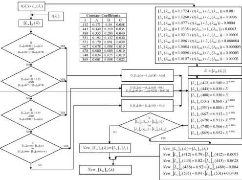
independent of the model of diffuse transmittance proposed by Gordon and Wang (1994) and Wang (1999). A set of equations determined from this scheme can be used to con-vert [Lw(λi)]Nvalues to new [Lw(λi)]Nvalues as shown in Fig. 1. The new [Lw(λi)]N can easily be converted to nor-malized water-leaving reflectance through

[ρw(λi)]N= π F0(λi)

[Lw(λi)]N (20)

where F0 is the mean extraterrestrial solar irradiance. It

should be noted that many algorithms use remote sensing reflectance (Rrs=Lw/Ed, whereEdis the downward

irradi-ance just above the sea surface) rather than [ρw]N or [Lw]N (O’Reilly et al., 1998). However, to a good approximation [ρw]N=π Rrs (Gordon and Voss, 1999; Shanmugam and

Ahn, 2007a). It should be noted that these spectral mod-els and coefficients (Eqs. 4–17 and Fig. 1) of the CAAS algorithm described above are different from those of the SeaDAS scheme, and work well regardless of the nature of complex situations in different regions.

3 Data and methods

3.1 In-situ data

To assess efficacy of CAAS algorithm, the resultant prod-ucts of this algorithm and SeaDAS algorithm are compared with in-situ radiometric measurements (at key wavelengths) and chlorophyll concentrations obtained from the NOMAD database (NASA bio-Optical Marine Algorithm Data set, Werdell and Bailey, 2005) for different regions around the world. These data are high quality in-situ bio-optical datasets collected over a wide range of optical properties, trophic sta-tus, and geographical locations in open ocean waters, es-tuaries, and coastal waters. Despite these data encompass large samples, only few cruises data were used consisting of 57 radiometric and pigment measurements collected between 2003 and 2007 in various regional waters (Cruises TANK2, FLA KEYS, WFS, 2004, 2005, 2006 and 2007, for which Chl ranged from 0.15 to 5.9 mg m−3). Dates when satellite sampling for a given station was masked by clouds or af-fected by sensor digitization problems were excluded from the analysis.

3.2 Satellite data and processing

MODIS-Aqua Level 1A data (∼1 km pixel−1_{at nadir,}

  34  

835 

  836 

  837 

  838 

  839 

  840 

  841 

  842 

  843 

  844 

  845 

  846 

  847 

  848 

  849 

  850 

  851 

Fig. 1. Schematic representation of an iterative spectral matching scheme of the CAAS algorithm.

852 

853 

854 

855 

856 

857 

858 

859 

  860 

Fig. 1. Schematic representation of an iterative spectral matching scheme of the CAAS algorithm.

also obtained for assessing the performance of CAAS and SeaDAS algorithms. First, the MODIS L1A data that con-sisted of calibrated and scaled top of atmospheric radiances (Lt(λ)) were input to the SeaDAS atmospheric correction

code to output the Rayleigh-corrected (Lrc(λ))radiances at

all wavelengths. BothLt(λ) and Lrc(λ) were input to the

CAAS algorithm to retrieve the desired water-leaving radi-ance products. Before applying these corrections, an opera-tional cloud-masking scheme for all MODIS-Aqua data (ex-cept 4 December 2010 scene, which we discuss in a later section) was adopted to create flags over the cloud-covered regions. The resulting products were converted to the re-mote sensing reflectance (Rrs)and the pigment

concentra-tions were estimated using a Case 2 water bio-optical algo-rithm proposed by Aiken et al. (1995) (also found in Carder et al., 2003). This is called the “empirically-derived or “de-fault” algorithm which uses theRrs(488)/Rrs(551) ratio for

chlorophyll determination. A large number data used for deriving this algorithm came from riverine-influenced and coastal waters, and therefore resulted in a best fit

regres-sion with a set of coefficients as described in Table 1. The SeaDASRrsand their chlorophyll products were also derived

and examined in a similar way.

4 Results and discussion

4.1 Application to MODIS-Aqua imagery

4.1.1 Image comparisons

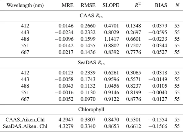
Table 1. Comparison of algorithm performances using MODIS-AquaRrs(from SeaDAS and CAAS algorithms) and coincidently measured (in situ)Rrs(NOMAD data sets). Note that the in-situ measurements are made at 412, 443, 490, 555 and 670 nm.

Wavelength (nm) MRE RMSE SLOPE R2 BIAS N

CAASRrs

412 0.0146 0.2660 0.4701 0.1348 0.0379 55

443 −0.0234 0.2332 0.8029 0.2697 −0.0595 55

488 −0.0096 0.1599 1.1417 0.6601 −0.0233 55

551 0.0142 0.1455 0.8802 0.7207 0.0344 55

667 0.0217 0.1436 0.8392 0.7776 0.0527 55

SeaDASRrs

412 0.0123 0.2339 0.6261 0.3065 0.0318 55

443 −0.0058 0.1743 0.9596 0.5571 −0.0149 55

488 0.0043 0.1132 1.0456 0.8237 0.0105 55

551 −0.0016 0.1130 0.9146 0.8199 −0.0040 55

667 0.0052 0.0970 0.9122 0.8776 0.0127 55

Chlorophyll

CAAS Aiken Chl 4.2947 0.3807 0.8470 0.5301 −0.1554 55 SeaDAS Aiken Chl 4.3279 0.3340 0.8653 0.6612 −0.1566 55

Aiken Chl = 10(0.2818−2.783×R+1.863×R2−2.387×R3)_{, whereR}=log₁₀[Rrs(488)/Rrs(551)]

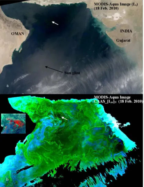
sun glint in the central part and furthermore contaminated by haze, desert dust and strip of clouds. It is apparent that the density of this mineral (desert) dust is not uniform, and it is very strong in the vicinity of desert coasts and across the Arabian Sea. The corresponding true colour composite atmospherically corrected by the CAAS algorithm removes all these effects (Fig. 2b) and becomes more comprehensive to demonstrate that large-scale Noctiluca miliaris blooms de-veloped in the Gulf of Oman and mesoscale eddies that pop-ulated the western Arabian Sea during the winter monsoon contributed to the genesis and dispersal of these blooms from the Gulf of Oman into the central Arabian Sea (Gomes et al., 2008). The green features in the nearshore and offshore wa-ters are well characterized by weaker radiances in the blue band, while the brighter features relate to highly reflective materials along the coastal areas (especially Gujarat in the eastern Arabian Sea) caused by strong radiance in the green band. These episodic high values of radiance in the green are indicative of high particle loads supporting its use as a plume indicator with satellite data sets (Otero and Siegel, 2004).

A true colour MODIS-Aqua image (4 December 2010) around Korea also displays intense Yellow dust aerosols (from Gobi desert) covering a vast space with a pronounced variability over the YS and ECS and around Korea (Fig. 3a). It becomes evident that the estuary of Yangtze River and Bo-hai Sea are the most turbid sea areas in this region, where the SS concentration can go up to 30 kg m−3and water-leaving radiance at 765 nm up to 4.5 mW cm−2µm−1sr−1 (Xian-qiang et al., 2004). As a consequence, most of the scene,

which was derived with the SeaDAS algorithm, is flagged out due to these difficult conditions (Fig. 3b). This prob-lem could also be linked to the cloud-masking threshold with SeaDAS that often identifies the hazy and turbid atmosphere as clouds (Hu, 2009). Thus, the present threshold was re-laxed in our data processing and useful ocean colour retrieval could be achieved with the CAAS algorithm. As expected, the CAAS performed very well in removing complex atmo-spheric conditions and achieving rather more realistic spa-tial structure in water-leaving radiance maps for the entire area which was previously flagged out by the SeaDAS algo-rithm. The spatial structures observed in Fig. 3c also cor-relate well with known SS distributions. It should be noted that the threshold for cloud detection needs to be enhanced for more complex water applications, because the assump-tion of low near-infrared water-leaving radiance is no longer valid (Ruddick et al., 2000).

4.1.2 Spectral analysis

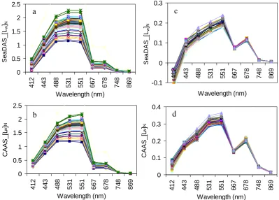
Spectral analysis is a very useful part to examine any conse-quences of the CAAS and SeaDAS algorithms on the spec-tral features ofLw(λ)retrieved from MODIS-Aqua data. For

this preliminary comparison, a group of [Lw]N andLrc(λ)

spectra collected from two locations (marked by arrows in Figs. 2b and 3c) for both CAAS and SeaDAS algorithms are shown in Fig. 4 (a–c: for bloom waters in the northern Ara-bian Sea; d–f: for SS waters in the Korean Southwest Sea). It is important to note that theLrc(λ)values of bloom waters

Fig. 2.

* Replace the previous one with this figure (see a white arrow inserted on the top panel).

Fig. 2. MODIS-Aqua true colour composite imagery (18 Febru-ary 2010) for the Arabian Sea generated from the total radiances at 443, 551 and 488 nm (B253) (a) and the corresponding water-leaving radiance imagery from the CAAS algorithm (b). Subset im-age generated from the [Lw]Nat 748, 678 and 667 nm (Band 876) are displayed on the left side of the bottom panel confirming highly concentrated patches of algal blooms in the northern central Ara-bian Sea.

NIR (748 nm) similar to land vegetation. This ocean feature is a typical of highly concentrated or floating algal blooms (see a subset on Fig. 2b). Most of these spectra present al-ways non-zero values at the NIR bands and near-zero values (sometime negatives) at the short-wavelengths bands (e.g. 412 nm), meaning that an assumption of zeroρw at NIR or

an updated SeaDAS algorithm with a NIR correction scheme can be easily invalidated by these conditions. Comparisons between the CAAS and SeaDAS algorithms clearly demon-strate large anomalous differences in their [Lw]Nspectra col-lected from waters with dense algal blooms, i.e. large distor-tions in [Lw]Nstructures with high negative values across the wavebands revealed by the SeaDAS algorithm. According to the true colour composite image in Fig. 2a (around a white arrow mark), the atmosphere was rather clear on 18 Febru-ary 2010 but the SeaDAS algorithm produced [Lw]N val-ues reaching as low as−0.64 mW cm−2µm−1sr−1at 412 nm and −0.23 mW cm−2µm−1sr−1 at 667 nm. The dramatic

anomalous negative [Lw]N values could be attributed to the black-pixel assumption or inadequacy of the NIR correction scheme with the SeaDAS algorithm. The consequence of these problems could also be observed in a recent study, where the MODIS-Aqua derived Chl and nLw(443) data over

Arabian Sea waters were flagged out by the SWIR and NIR-SWIR schemes due to complex conditions (see Fig. 6 in Wang, 2009). This indicates that a simple relaxation of the black pixel assumption alone is not sufficient to improve re-trievals of [Lw]Nat the shorter wavelengths, and other com-ponents of the processing chain may also require refinement if reliable [Lw]N in this domain are to be achieved (Rud-dick et al., 2000). By contrast, the CAAS algorithm out-performed the SeaDAS algorithm in terms of successfully removing most atmospheric effects and producing non-zero [Lw]N values for these dense blooms. It becomes conspicu-ous that with increasing absorption at 443 nm, a primary peak shifts from blue to green and a secondary peak from red to NIR in Fig. 4c. The secondary peak suggests that the con-centrations of dense or floating algal blooms can be possibly mapped and quantified with a suitable bio-optical algorithm combined with the CAAS algorithm.

Figure 4d–f shows the Rayleigh collected spectra and their corresponding [Lw]Nspectra obtained with the CAAS and SeaDAS algorithms in turbid waters around the Korean Southwest Sea (as indicated by arrow in Fig. 3c). Contrary to bloomed waters, the correlation between theLrc(λ) and

[Lw]N is noticeable in turbid waters, because these pixels

are relatively free of aerosols and dominated by SS concen-trations. Thus, there is consistency in [Lw]N structure

ob-tained with these algorithms, although the CAAS algorithm produced slightly low values across the wavelengths. Note that the effect of atmospheric correction with the SeaDAS al-gorithm on lowering radiance values is clearly seen in [Lw]N spectra at 412 nm, as opposed by the results of the CAAS al-gorithm (Fig. 4e and f).

  36

889 

890 

891 

892 

893 

894 

895 

896 

897 

898 

899 

900 

901 

902 

903 

904 

905 

906 

907 

908 

909 

910 

Fig. 3. MODIS-Aqua true colour composite image (4 Dec. 2010) for the East China Sea (ECS),

911 

Yellow Sea (YS), Bogai Sea (BS) and waters around Korea generated from the total radiances at 443,

912 

551 and 488nm (B253) (a) and the corresponding water-leaving radiances from the SeaDAS

913 

algorithm (b) and CAAS algorithm (c).

914 

915 

916 

c

MODIS-Aqua Image CAAS_[Lw]N (4 Dec. 2010)

b

MODIS-Aqua Image SeaDAS_[Lw]N (4 Dec. 2010)

a

KOREA

CHINA

MODIS-Aqua Image (Lt)

(4 Dec. 2010)

BS

YS

ECS

Algal blooms

Fig. 3. MODIS-Aqua true colour composite image (4 December 2010) for the East China Sea (ECS), Yellow Sea (YS), Bogai Sea (BS) and waters around Korea generated from the total radiances at 443, 551 and 488 nm (B253) (a) and the corresponding water-leaving radiances from the SeaDAS algorithm (b) and CAAS algorithm (c).

4.1.3 Aerosol analysis

To understand the potential causes of biased negative [Lw]N with the SeaDAS algorithm, aerosol radiances derived from MODIS-Aqua imagery of the Arabian Sea (18 Febru-ary 2010) were examined for a group of pixels encompass-ing bloomed, turbid and relatively clear waters. No com-parisons are presented here for typical Case 1 waters since the CAASLaand SeaDAS La for these waters had

excep-tionally good correlations (R2∼=1) at all wavelengths. Scat-ter plots in Fig. 6 show the relationship between CAASLa

and SeaDASLa, wherein the dark colour cluster represents

aerosol radiances calculated using Eqs. 4–6 (Lrc as input)

and the grey colour cluster represents aerosol radiances it-eratively calculated using Eqs. (4)–(8) (with correctedLaat

NIR bands as input). Interestingly, there is a tight, linear

relationship between CAASLaand SeaDASLa at 748 and

  37   917    918    919    920    921    922    923    924    925    926    927    928    929    930    931    932    933    934    935    936    937    938 

Fig. 4. Rayleigh-corrected a(Lt-Lr) and water-leaving radiance spectra [Lw]N for intense algal bloom 939 

waters of the Arabian Sea (a-c) and turbid waters of the Korean Southwest Sea (d-f), obtained from

940 

MODIS-Aqua imageries (a-c: 18 Feb. 2010; d-f: 4 Dec. 2010) using the SeaDAS and CAAS

941 

algorithms. Locations are indicated in the corresponding MODIS-Aqua data (Fig. 2b and Fig. 3c).

942    943    944  0 0.1 0.2 0.3 0.4 0.5

412 443 488 531 551 667 678 748 869

Wavelength (nm) CA A S _ [L w] N -0.1 0 0.1 0.2 0.3 0.4 0.5 0.6 0.7

412 443 488 531 551 667 678 748 869

Wavelength (nm) L t -L r -0.8 -0.6 -0.4 -0.2 0 0.2 0.4

412 443 488 531 551 667 678 748 869

Wavelength (nm) SA C _ [L w ] N

a

b

c

412 443 488 531 551 667 678 748 869

Wavelength (nm) CA A S _ [L w] N 0 0.3 0.6 0.9 1.2 1.5 1.8 2.1

412 443 488 531 551 667 678 748 869

Wavelength (nm) SA C _ [L w] N 0 0.5 1 1.5 2 2.5

412 443 488 531 551 667 678 748 869

Wavelength (nm) L t-L r

d

e

f

Fig. 4. Rayleigh-corrected(Lt−Lr)and water-leaving radiance spectra [Lw]Nfor intense algal bloom waters of the Arabian Sea (a)–(c) and turbid waters of the Korean Southwest Sea (d)–(f), obtained from MODIS-Aqua imageries (a–c: 18 February 2010; d–f: 4 December 2010) using the SeaDAS and CAAS algorithms. Locations are indicated in the corresponding MODIS-Aqua data (Figs. 2b and 3c).

algal blooms at these wavelengths (see in Fig. 4a). Gains in aerosol radiances (especially at 412–488 nm) for turbid waters confirm the presence of scattering sediments in these waters. The effect of this significant increase in aerosol ra-diances toward the short wavelengths is clearly seen in the negatively biased water-leaving radiances of the SeaDAS al-gorithm for bloomed waters (see in Fig. 4b). By contrast, the CAAS produced slightly higher aerosol radiances for turbid waters, but such gains were significantly reduced by remov-ing the near-infrared water signal at 748 and 865 nm through Eqs. (4)–(8).

The Arabian Sea is known to be caused by frequent algal blooms and strongly absorbing aerosols (mineral dust from adjacent deserts). The most essential distortions inLw

val-ues are revealed in such conditions prevailing together, and are therefore completely discarded in the processing proce-dure together with ordinary atmospheric clouds, if the dust density is too high. Figure 7 shows the example of compar-ison between the SeaDAS-derivedLa(λ)and CAAS-derived

La(λ)for the above conditions in the Arabian Sea. Clearly,

the CAAS-derived La increases from 869 to 488 nm and

  38   945    946    947    948    949    950    951    952    953    954    955    956    957    958    959 

Fig. 5. Comparison of the water-leaving radiance spectra [Lw]N for turbid waters (a-b) and algal bloom

960 

waters (c-d) obtained from MODIS-Aqua image (4 Dec. 2010) using the SeaDAS and CAAS 961 

algorithms. These spectra are from bloom and turbid waters in the East China Sea (see arrow marks in 962  Fig. 3c). 963  964    965    966    967    968    969    970    971    972  0 0.1 0.2 0.3 0.4

412 443 488 531 551 667 678 748 869

Wavelength (nm) CA A S _ [L w] N 0 0.5 1 1.5 2 2.5

412 443 488 531 551 667 678 748 869

Wavelength (nm) CA A S _ [L w] N 0 0.5 1 1.5 2 2.5

412 443 488 531 551 667 678 748 869

Wavelength (nm) SA C _ [L w ] N -0.1 0 0.1 0.2 0.3

412 443 488 531 551 667 678 748 869

Wavelength (nm) SA C _ [L w] N

a

b

c

d

Fig. 5. Comparison of the water-leaving radiance spectra [Lw]N for turbid waters (a)–(b) and algal bloom waters (c)–(d) obtained from MODIS-Aqua image (4 December 2010) using the SeaDAS and CAAS algorithms. These spectra are from bloom and turbid waters in the East China Sea (see arrow marks in Fig. 3c).

mineral aerosols (non-absorbing aerosols not shown because of their highLavalues suppressing the spectral variability of

absorbing case). Note that a pronounced lowLaat 412 nm is

the result of these aerosols. However, different spectral fea-tures inLa(λ)are derived from the SeaDAS algorithm which

are rather steadily increasing from 869 to 443 nm with a slight low at 412 nm. These unrealisticLa(λ)values

eventu-ally lead to an excessive correction in the violet–green wave-lengths, which in turn result in large errors in chlorophyll retrieval from MODIS-Aqua data or discarding of such data in case of the higher dust density (Fig. 4a–c and within cir-cles in Fig. 10). Many similar data sets for the Arabian Sea from different periods were processed showing a lot of anal-ogous results that confirm the existence of negative spatial and temporal correlation between SeaDASLwandτawhen

the aforesaid conditions occur. 4.1.4 Sun glint analysis

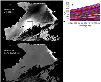
Figure 8a shows a typical distribution of sun glint measured at 551 nm and confirms that the glint contaminated portion of the image extends across the bloomed region in the cen-tral Arabian Sea. Of importance is the speccen-tral contribution. Figure 8b shows the relative sun glint radiances for pixels within the box in Fig. 8a. The relative sun glint radiances

in-crease with increasing wavelength and obvious is its strong contribution in the NIR, where the bands used for atmo-spheric correction are positioned. It is even much higher (at longer wavelengths) than the radiance caused by atmospheric molecule scattering. The corresponding water-leaving radi-ance image shown in Fig. 8c indicates that the CAAS algo-rithm definitely improved ocean colour retrieval for the pix-els contaminated by sun glint. Furthermore, the CAAS al-gorithm was able to recover more areas which were previ-ously masked or having erroneous values produced by the SeaDAS algorithm. This is apparent in their Chl-a images as discussed in the later section. These results imply that the current model works well as long as the sun glint contribu-tion does not fully contaminate the water signal that reaches a satellite sensor.

4.2 Validation of the CAAS algorithm

214  P. Shanmugam: CAAS: an atmospheric correction algorithm for the remote sensing of complex waters

1 

2 

3

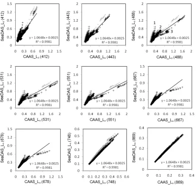
Fig. 6. Scatter plots of the CAAS retrieved La versus the SeaDAS retrieved La from

MODIS-Aqua imagery (18 Feb. 2010) in bloomed, turbid and relatively clear waters of the Arabian Sea.

Fig. 6. Scatter plots of the CAAS retrievedLaversus the SeaDAS retrievedLafrom MODIS-Aqua imagery (18 February 2010) in bloomed, turbid and relatively clear waters of the Arabian Sea.

1001   

1002   

1003   

1004   

1005   

1006   

1007   

1008   

1009   

1010 

Fig. 7. Comparison of aerosol radiances derived from MODIS-Aqua imagery of bloomed waters of

1011 

the Arabian Sea (18 February 2010) using the SeaDAS and CAAS algorithms.

1012   

1013   

1014   

1015   

1016   

1017   

1018   

1019   

1020   

1021   

1022   

1023   

1024   

1025   

1026   

1027   

1028 

0 0.05 0.1 0.15 0.2 0.25

412 443 488 531 551 667 678 748 869

Wavelength (nm)

C

AAS

_

L

a

0 0.05 0.1 0.15 0.2 0.25 0.3 0.35 0.4

412 443 488 531 551 667 678 748 869

Wavelength (nm)

Se

a

D

AS

_

L

a

Fig. 7. Comparison of aerosol radiances derived from MODIS-Aqua imagery of bloomed waters of the Arabian Sea (18 February 2010) using the SeaDAS and CAAS algorithms.

  41

1029 

1030 

1031 

1032 

1033 

1034 

1035 

1036 

1037 

1038 

1039 

1040 

1041 

1042 

1043 

1044 

1045 

Fig. 8. Rayleigh-corrected radiance (a), sun glint spectra (b) and water-leaving radiance (c) from

1046 

MODIS-Aqua imagery of 18 Feb. 2010 (Arabian Sea) processed using the CAAS algorithm.

1047 

1048 

1049 

1050 

1051 

1052 

1053 

1054 

1055 

412450 500 550 600 650 700 750 800 850 0.00

0.05 0.10 0.15 0.20 0.25 0.30 0.35 0.40 0.45

Lsg

(

λ

)

Wavelength (nm)

18‐2‐2010 

CAAS_[Lw]N(551) 

18‐2‐2010 

Lt‐Lr (551) 

a

c

b

Fig. 8. Rayleigh-corrected radiance (a), sun glint spectra (b) and water-leaving radiance (c) from MODIS-Aqua imagery of 18 February 2010 (Arabian Sea) processed using the CAAS algorithm.

the SeaDAS algorithm produced probable positiveLw

vues. The results of applying the CAAS and SeaDAS al-gorithms to 55 matchups data are shown in the scatterplots (Fig. 9) and their corresponding statistics in Table 1. Interest-ingly, theRrsvalues from the CAAS and SeaDAS algorithms

are approximately aligned closer to the 1:1 line with respect to in-situ data at all wavelengths (except 412 and 667 nm). The lowRrsvalues at 667 nm produced by the SeaDAS

algo-rithm are erroneous and result in part from not fully taking into account that water-leaving radiance in the NIR. For clear waters the retrieval error of the CAAS algorithm is noticeable at 412 nm (few data points below the 1:1 line towards the higher end), and could be due to the added spectral variabil-ity of the atmospheric spectral models. On the other hand, the CAAS algorithm generated slightly higher water-leaving ra-diances at the longer wavelength (667 nm), but there was no data to confirm this. Because water absorption is expected to dominate the water signal at longer wavelengths and thus re-sult in essentially black waters at NIR, the SeaDAS returned nearly the same as the in-situ water-leaving radiance and the magnitude of the discrepancy is therefore less remark-able in relatively clear waters (thus slightly better statistics). This demonstrates that in clear waters the SeaDAS algorithm might be a better option for atmospheric correction.

The impact of atmospheric correction on retrievals of pig-ment concentration was also studied with a Case 2 water

bio-optical algorithm developed by Aiken et al. (1995). This sim-ple band ratio algorithm relying on 488 and 551 nm bands is more suitable for optically complex waters since these bands are not much influenced by the constituents other than phy-toplankton such as dissolved organic matter and suspended matter. Despite the limited number of observations at high chlorophyll regions, the regional matchups dataset confirms that the chlorophyll concentrations derived from CAASRrs

are better consistent with measured chlorophyll data than those derived from SeaDAS Rrs. In moderately complex

waters with Chl 2–6 mg m−3, an overestimation of chloro-phyll by the SeaDAS algorithm is obvious simply because of the enhanced water signal interfering with the NIR scheme with this algorithm. Such an effect is minimised in chloro-phyll from the CAASRrs, with a MRE 4.29, RMSE 0.38,

slope 0.847, R2 0.53 and bias−0.155. The mean chloro-phyll concentration for all 55 matchup data is 1.71 mg m−3 (in situ), 2 mg m−3(CAAS), and 2.3 mg m−3(SeaDAS). 4.3 Application to MODIS-Aqua imagery

  42   1056    1057    1058    1059    1060    1061     1062    1063    1064    1065    1066    1067    1068     1069    1070    1071    1072    1073    1074  1075  1076  1077  1078 

Fig. 9. Comparison of in situ measurements of the remote sensing reflectance with coincident 1079 

MODIS-Aqua spectra (from various regional waters) from the SeaDAS and CAAS algorithms. The 1080 

Chl-a concentrations retrieved from the Aiken bio-optical algorithm using CAAS_Rrs and SeaDAS Rrs

1081 

are shown in the bottom-right corner panel. 1082    1083    1084    1085  0.0001 0.001 0.01 0.1

0.0001 0.001 0.01 0.1

In situ Rrs (412)

MO D IS R rs ( 412) 0.0001 0.001 0.01 0.1

0.0001 0.001 0.01 0.1

In situ Rrs (443)

MO

D

IS

R

rs (

443)

0.0001 0.001 0.01 0.1

0.0001 0.001 0.01 0.1

In situ Rrs (488)

MO D IS R rs ( 488) 0.0001 0.001 0.01 0.1

0.0001 0.001 0.01 0.1

In situ Rrs (551)

MO

D

IS

R

rs (

551)

0.0001 0.001 0.01 0.1

0.0001 0.001 0.01 0.1

In situ Rrs (667)

MO D IS R rs ( 667) 0.01 0.1 1 10 100

0.01 0.1 1 10 100

In situ Chl-a

M O DI S Ch l-a CAAS_Aiken_Chl SeaDAS_Aiken_Chl

Fig. 9. Comparison of in situ measurements of the remote sensing reflectance with coincident MODIS-Aqua spectra (from various regional waters) from the SeaDAS and CAAS algorithms. The Chl-aconcentrations retrieved from the Aiken bio-optical algorithm using CAASRrs and SeaDASRrsare shown in the bottom-right corner panel.

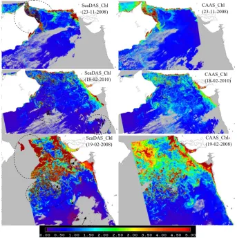
resulted in inaccurate, overestimated (often >30 mg m−3 in offshore patches of blooms) and spatially homogeneous chlorophyll in highly bloomed regions, where no field obser-vations showed values in excess of 30 mg m−3. A re-analysis of the same data using the present CAAS algorithm shows substantial improvements. In particular, nearly all of the ex-cessive Chl retrievals have been corrected and the spatial pat-terns in algal blooms are more realistic. It is also evident that some coastal turbid features (indicated by an arrow mark on the 23 November 2008 image) are captured with very high chlorophyll concentrations, which is an indication of the at-mospheric correction failure meaning that the signal is over corrected for the atmosphere. However, the CAAS algorithm seems to suppress such features by means of producing re-alistic Lw spectra. The atmospheric correction failure in

bloomed waters (negativeLw(λ)values) is primarily due to

the fact that waters containing large accumulations of algal matters have a relatively strong water-leaving radiance in the near-infrared bands (as evident in Fig. 4 left panels), while at the same time are absorbing strongly in the blue green do-main, which leads to possible errors in the atmospheric cor-rection and underestimation ofLw(λ)in the blue and green

  43  

1086 

  1087 

  1088 

  1089 

  1090 

  1091 

  1092 

  1093 

  1094 

  1095 

  1096 

  1097 

  1098 

  1099 

  1100 

  1101 

  1102 

  1103 

  1104 

  1105 

  1106 

  1 

  1108 

Fig. 10. Chlorophyll concentrations derived from the Aiken Case 2 bio-optical algorithm using 1109 

MODIS-Aqua derived remote sensing reflectances from the SeaDAS and CAAS algorithms. 1110 

  1111 

SeaDAS_Chl (19-02-2008)

CAAS_Chl (19-02-2008) SeaDAS_Chl

(18-02-2010) CAAS_Chl _(18-02-2010)

SeaDAS_Chl (23-11-2008)

CAAS_Chl (23-11-2008)

Fig. 10. Chlorophyll concentrations derived from the Aiken Case 2 bio-optical algorithm using MODIS-Aqua derived remote sensing reflectances from the SeaDAS and CAAS algorithms.

recovered with the more realistic spatial features consistent with the adjacent regions. In case of clear oceanic waters, the magnitude of chlorophyll signal is nearly the same for both the algorithms suggesting not much impact of the atmo-sphere correction on the ratio of signal magnitudes at blue-green bands.

4.4 Implications for the Geostationary Ocean Colour Imager (GOCI)

In comparison with open ocean applications, coastal appli-cations involving phenomena that vary on shorter space and time scales demand a simultaneous increase in spatial and temporal resolution. The geostationary ocean colour imager such as the GOCI (currently providing data for ECS, YS, ES and Korean waters) has a unique capability to observe the ocean and coastal waters with high spatial resolution (500 m), very high temporal resolution (refresh rate: 1 h) and spectral resolution similar with MODIS-Aqua (Shanmugam and Ahn, 2007b). Such sensors are capable of detecting, monitoring, and predicting short term and regional oceanic

5 Summary and conclusions

The direct application of the SeaDAS algorithm yields ex-cessive errors in retrieved water-leaving radiance and bio-physical products in complex waters (likely due to overes-timation ofLa+Lrain the visible and thus reduction inLw

there which appears as an elevated pigment concentration). The principal difficulty in these waters is:

1. The adequacy of aerosol models is presently difficult to judge. This holds true for mineral dust aerosols (from deserts) because their absorption can seriously reduce La+Lra in the visible and their vertical distribution

profoundly influences the TOA radiance in the visible (especially in the blue) (Gordon, 1997; Moulin et al., 2001). Moreover, the absorption properties are very dif-ficult to determine on the basis of the observations of La+Lrain the NIR which means that in-situ

measure-ments in the visible are required for correction. How-ever, in the visible (especially blue)Lw can be

signifi-cant, and cannot be estimated a priori (Gordon, 1997). 2. The errors involved in extrapolating aerosol reflectance

to visible bands are considerably higher and this may require a more realistic method (Ruddick et al., 2000). 3. Assumption of negligible water-leaving radiance in the

NIR is not valid in complex waters, as high SS loads and phytoplankton will contribute NIR radiance (Arnone et al., 1998; Siegel et al., 2000; Ruddick et al., 2000). 4. Difficulty in dealing with highly turbid atmosphere that

is presently considered as the “high aerosol” and is masked whenτa(869)>0.4 (Robinson et al., 2003).

5. Because of the difficulty in removing sun glint, the TOA sun glint radianceT (λ). Lg(λ)is mostly masked out and residual contamination is corrected based on a model of sea surface slope distribution (Wang and Bai-ley, 2001). Consequently, the criteria used in points 4 and 5 lead to a tremendous loss of information for ocean colour work.

6. Although modifications to point 3 (i.e. “non-zeroLwin

the NIR” based on in-water models and spatial homo-geneity assumption; Arnone et al., 1998; Siegel et al., 2000; Ruddick et al., 2000; Hu et al., 2000) show no-ticeable improvements in turbid waters, problems are still encountered in highly bloomed waters and could be attributed to inadequacy of aerosol models as stated in points 1 and 2. As evident in Figs. 2, 3 and 10 (true colour composite not shown here), many assump-tions regarding aerosols are invalidated because of their strong diversity and compositional changes across these regions.

Many of the above properties can indeed be derived in the whole spectrum of ocean colour solely from a knowledge of

the total and Rayleigh-corrected radiances, and that possibil-ity has been developed in detail within the framework of the CAAS algorithm that makes no use of ancillary parameters. This algorithm has been tested with MODIS-Aqua images of optically very complex waters in the Arabian Sea and around Korea and with in-situ measurements of the remote sensing reflectance and Chl concentrations in various regional wa-ters. The new algorithm shows promise in dealing with the diversity and variability of aerosols and strong sun glint pat-terns, and produces more realistic spatial structures in water-leaving radiance maps as well as positive water-water-leaving ra-diance for all visible bands, whereas the SeaDAS algorithm yields significantly lowerLw (often negativeLwat 412 nm)

in highly turbid waters and unphysical negativeLwat many

wavelengths in highly bloomed waters. A clear underestima-tion ofLwwith increasing error toward lower wavelengths is

typical of excessive aerosol path radiance removal. Further-more, the spatial patterns previously masked by the SeaDAS algorithm in the sun glint contaminated and strong aerosol regions are successfully recovered by the CAAS algorithm. It was noted that CAAS returns slightly lowLw at 412 nm

and highLwat 667 and 678 nm especially for clear waters.

Nevertheless, the spectral form is still well produced by this algorithm at 667 and 678 nm that allows accurate measure-ments of the fluorescence light height above the background between 667 nm and 748 nm using a baseline method (Ab-bott and Letelier, 1999; Ahn and Shanmugam, 2007). Also, our analysis shows that the retrieved pigment concentrations with CAAS algorithm are more realistic than those derived with the SeaDAS algorithm, suggesting its practical utility for ocean colour applications in complex waters.

The results further suggest that the CAAS algorithm is an alternative correction scheme to process ocean colour im-agery in the presence of sun glint and strong aerosols (e.g. yellow dust). Though the algorithm has been described in the context of MODIS-Aqua imagery, it can be applied rather generally to other satellite-based and probably also airborne ocean colour sensors. The directions for further research in-clude a more detailed validation of this algorithm with large in-situ datasets from highly turbid and productive waters and an attempt to tune it to have a wider applicability.

Acknowledgements. This work was supported by grants from the

Korean Ocean Research and Development Institute (KORDI), Ko-rea (No. OEC/10-11/101/KORD/PSHA). The author gratefully ac-knowledges the NASA Ocean Biology Processing Group for mak-ing available the global, high quality in situ bio-optical (NOMAD) dataset as well as the LAC MODIS-Aqua data to this study. The author is indebted to the three anonymous reviewers for their con-structive comments and recommendations.

References

Abbott, M. R. and Letelier, R. M.: ATBD 22-Chlorophyll Fluo-rescence, NASA Algorithm Theoretical Basis Document, http: //modis.gsfc.nasa.gov/data/atbd/atbd mod22.pdf, 1999. Ahn, Y. H. and Shanmugam, P.: Derivation, analysis of the

fluo-rescence algorithms to estimate chlorophyll a concentrations in ocean waters. Journal of Optics A: Pure, Appl. Optics, 9, 352– 362, 2007.

Aiken, J., Moore, G. F., Trees, C. C., Hooker, S. B., and Clark, D. K.: The SeaWiFS CZCS-type pigment algorithm, in: SeaWiFS Technical Report Series, vol. 29, edited by: Hookerm S. B. and Firestonem E. R., Goddard Space Flight Center, Greenbelt, MD, 1995.

Amin, R., Gilerson, A., Zhou, J., Gross, B., Moshary, F., and Ahmed, S.: Impacts of Atmospheric Corrections on Algal Bloom Detection Techniques. Eighth Conference on Coastal Atmo-spheric, Oceanic Prediction, Processes, USA, 2009.

Arnone, R. A., Martinolich, P., Gould, R. W., Stumpf, R., and Ladner, S.: Coastal optical properties using SeaWiFS, presented at Ocean Optics XIV Conference, Kailua-Kona, Hawaii, Ocean Optics XIV, Washington, D.C., 1998.

Carder, K. L., Chen, F. R., Lee, Z., Hawes, S. K., and Cannizzaro, J. P.: MODIS Ocean Science Team Algorithm Theoretical Basis Document, ATBD 19, Case 2 Chlorophyll a, version 7, http:// modis.gsfc.nasa.gov/data/atbd/atbd mod19.pdf, 2003.

Coppin, P. R. and Bauer, M. E.: Processing of multi-temporal L,sat TM imagery to optimize extraction of forest cover change fea-tures, IEEE Trans. Geosci. Remote Sens., 32, 918–927, 1994. Doerffer, R., Schiller, H., Fischer, J., Preusker, R., and Bouvet, M.:

The impact of sun glint on the retrieval of water, parame., Proc. of the 2nd MERIS (A) ATSR User Workshop, Frascati, Italy, 2008. Gomes, H. R., Goes, J. I., Matondkar, S. G. P., Parab, S. G., Al-Azri, A. R. N., and Thoppil, P. G.: Blooms of Noctiluca miliaris in the Arabian Sea-An in situ, satellite study, Deep Sea Res. Part I., 55, 751–765, doi:10.1016/j.dsr.2008.03.003, 2008.

Gordon, H. R.: Atmospheric correction of ocean colour imagery in the Earth Observing System era, J. Geophys., 102, 17081–17106, 1997.

Gordon, H. R. and Voss, K. J.: MODIS Normalized Water leaving Radiance Algorithm Theoretical Basis Document, University of Miami, USA, 1999.

Gordon, H. R. and Wang, M.: Surface Roughness Considerations for Atmospheric Correction of Ocean Colour Sensors. 1: The Rayleigh Scattering Component, Appl. Optics, 31, 4247–4260, 1992.

Gordon, H. R. and Wang, M.: Retrieval of water-leaving radiance, aerosol optical thickness over the oceans with SeaWiFS: a pre-liminary algorithm, Appl. Optics, 33, 443–452, 1994.

Gordon, H. R., Brown, O. B., and Evans, R. H.: Exact Rayleigh scattering calculations for use with the Nimbus-7 Coastal Zone Colour Scanner, Appl. Optics, 27, 862–871, 1988.

Hooker, S. B., Esaias, W. E., Feldman, G. C., Gregg, W. W., and McClain, C. R.: SeaWiFS Technical Report Series vol 1, An overview of SeaWiFS, Ocean Colour, NASA Technical Mem-orandum, 104566, 1992.

Hu, C.: A novel ocean colour index to detect floating algae in the global oceans, Remote Sens. Environ., 113, 2118–2129, 2009. Hu, C., Carder, K. L., and Muller-Karger, F. E.: Atmospheric

cor-rection of SeaWiFS imagery over turbid waters: a practical

ap-proach, Remote Sens. Environ., 74, 195–206, 2000.

Hwang, P. and Shemdin, O.: The Dependence of Sea-Surface Slope on Atmospheric Stability, Swell Conditions, J. Geophys. Res., 93, 13903–13912, 1988.

Kay, S., Hedley, J. D., and Lavender, S.: Sun Glint Correction of High, Low Spatial Resolution Images of Aquatic Scenes: a view of Methods for Visible , Near-Infrared Wavelengths, Re-mote Sens., 1, 697–730, doi:10.3390/rs1040697, 2009.

Koepke, P.: Effective reflectance of oceanic whitecaps, Appl. Op-tics, 23, 1816–1824, 1984.

Lavender, S. J., Pinkerton, M. H., Moore, G. F., Aiken, J., and Patissier, D. B.: Modification to the atmospheric correction of SeaWiFS ocean colour images over turbid waters, Cont. Shelf Res., 25, 539–555, 2005.

Li, L. P., Fukushima, H., Frouin, R., Mitchell, B. G., He, M. X., Uno, I., Takamura, T., and Ohta, S.: Influence of submicron ab-sorptive aerosol on SeaWiFS-derived marine reflectance during ACE-Asia, J. Geophys. Res., 108, AAC 13-1 AAC 13-6, 2003. M´elin, F., Zibordi, G., and Djavidnia, S.: Development, validation

of a technique for merging satellite derived aerosol optical depth from SeaWiFS, MODIS, Remote Sens. Environ., 108, 436–450, 2007.

Moulin, C., Gordon, H. R., Banzon, V. F., and Evans. R. H.: As-sessment of Saharan dust absorption in the visible from SeaWiFS imagery, J. Geophys. Res., 106, 18239–18249, 2001.

Nobileau, D. and Antoine, D.: Detection of blue-absorbing aerosols using near infrared, visible (ocean colour) remote sensing obser-vations, Remote Sens. Environ., 95, 368–387, 2005.

O’Reilly, J. E., Maritorena, S., Mitchell, B. G., Siegel, D. A., Carder, K., Garver, S. A., Kahru, M., and McClain, C.: Ocean colour algorithms for SeaWiFS, J. Geophys. Res., 103, 937–953, doi:10.1029/98JC02160, 1998.

Otero, M. P. and Siegel, D. A.: Spatial, temporal characteristics of sediment plumes, phytoplankton blooms in the Santa Barbara Channel, Deep Sea Res., Part II., 51, 1139–1149, 2004. Robinson, W. D., Franz, B. A., Patt, F. S., Bailey, S. W., and

Werdell, P. J.: Masks, flags updates, SeaWiFS Postlaunch Tech-nical Report Series, NASA Tech. Memo, 206892, 2003. Ruddick, K. G., Ovidio, F., and Rijkeboer, M.: Atmospheric

cor-rection of SeaWiFS imagery for turbid coastal and inland waters, Appl. Optics, 39, 897–913, 2000.

Shanmugam, P. and Ahn, Y. H.: New atmospheric correction tech-nique to retrieve the ocean colour from SeaWiFS imagery in complex coastal waters, Journal of Optics A: Pure, Applied Op-tics, 9, 511–530, 2007a.

Shanmugam, P. and Ahn, Y. H.: Reference solar irradiance spectra and consequences of their disparities in remote sens-ing of the ocean colour, Ann. Geophys., 25, 1235–1252, doi:10.5194/angeo-25-1235-2007, 2007b.

Shanmugam, P., Ahn, Y. H., and Ram, P. S.: SeaWiFS sensing of hazardous algal blooms, their underlying physical mechanisms in shelf-slope waters of the Northwest Pacific during summer, Remote Sens. Environ., 112, 3248–3270, 2008.

Siegel, D. A., Wang, G. M., Maritorena, S., and Robinson, W.: At-mospheric correction of satellite ocean colour imagery: the black pixel assumption, Appl. Optics, 39, 3582–3591, 2000.

3228, doi:10.1029/2001JC000965, 2002.

Song, C., Woodcock, C. E., Seto, K. C., Lenney, M. P., and Ma-comber, S. A.: Classification , change detection using L,sat TM data: when , how to correct atmospheric effects?, Remote Sens. Environ., 75, 230–244, 2000.

Stumpf, R. P., Culver, M. E., Tester, P. A., Tomlinson, M., Kirkpa-trik, G. J., Pederson, B. A., Truby, E., Ransibrahmanakul, V., and Soracco, M.: Monitoring Karenia brevis blooms in the Gulf of Mexico using satellite ocean colour imagery, other data, Harm-ful Algae, 2, 147–160, 2003.

Wang, M.: A sensitivity study of the SeaWiFS atmospheric correc-tion algorithm: effects of spectral b, variacorrec-tions, Remote Sens. Environ., 67, 48–59, 1999.

Wang, M. and Bailey, S.: Correction of the sun glint contamination on the SeaWiFS ocean, atmosphere products, Appl. Optics, 40, 4790–4798, 2001.

Wang, M. and Shi, W.: The NIR–SWIR combined atmospheric cor-rection approach for MODIS ocean colour data processing, Op-tics Express, 15, 15722–15733, 2007.

Werdell, P. J. and Bailey, S. W.: An improved in-situ bio-optical data set for ocean colour algorithm development, satellite data product validation, Remote Sens. Environ., 98, 122–140, 2005. Werdell, P. J., Franz, B. A., and Bailey, S. W.: Evaluation of

short-wave infrared atmospheric correction for ocean colour remote sensing of Chesapeake Bay, Remote Sens. Environ., 114, 2238– 2247, 2010.

Xianqiang, H., Delu, P., and Zhihua, M.: Atmospheric correction of SeaWiFS imagery for turbid coastal and inland waters, Chinese Society of Oceanography, 23, 609–615, 2004.