The objective is to minimize the anticipated total cost rate by simultaneously optimizing the inventory level.

ISSN: 2320 –3242 (P), 2320 –3250 (online) Published on 30 April 2018

www.researchmathsci.org

DOI: http://dx.doi.org/10.22457/ijfma.v15n2a4

137

International Journal of

Analysis of Two-Echelon Inventory System with Two

Demand Classes with Partial Backlogging

R. Rohini and K. Krishnan*

PG & Research Department of Mathematics, Cardamom Planters’ Association College Bodinayakanur, Tamil Nadu, India -625513

*

Corresponding author. E-mail: [email protected]

Received 17 March 2018; accepted 21 April 2018

Abstract. This paper deals with a continuous review two-echelon inventory system with

two demand classes. Two echelon inventory systems consist of one retailer (lower echelon) and one distributor (upper echelon) handling a single finished product. The demand at retailer is of two types. The First type of demand is usual single unit and the second type is of bulk or packet demand. The arrival distribution for single and packet demands are assumed to be independent Poisson with rates λ1(>0) and λd (>0)

respectively. The operating policy at the lower echelon for the (s, S) that is whenever the inventory level drops to ‘s’ on order for Q = (S-s) items is placed, the ordered items are received after a random time which is distributed as exponential with rate µ>0. We assume that the demands occurring during the stock-out period are lost. The retailer replenishes the stock from the distributor which adopts (0, M) policy. The objective is to minimize the anticipated total cost rate by simultaneously optimizing the inventory level.

The joint probability disruption of the inventory levels at retailer and the distributor are obtained in the steady state case. Various system performance measures are derived and the long run total expected inventory cost rate is calculated. Several instances of numerical examples, which provide insight into the behavior of the system, are presented. Keywords: Markov inventory system, two-echelon, two demand classes, cost optimization. partial backlogging

AMS Mathematics Subject Classification (2010): 90B05

1. Introduction

138

reporting inventory status. In order to have clear inventory management, a company should not only focus on logistic management but also on sales and purchase management. Inventory management and control is not only the responsibility of the accounting department and the warehouse, but also the responsibility of the entire organization. Actually, there are many departments involved in the inventory management and control process, such as sales, purchasing, production, logistics and accounting. All these departments must work together in order to achieve effective inventory controls.

Study on multi-echelon systems are much less compared to those on single commodity systems. The determination of optimal policies and the problems related to a multi-echelon systems are, to some extent, dealt by Veinott and Wagner [22] and Veinott [23]. Sivazlian [20] discussed the stationary characteristics of a multi commodity single period inventory system. The terms multi-echelon or multi-level production distribution network and also synonymous with such networks (supply chain) when on items move through more than one steps before reaching the final customer. Inventory exist throughout the supply chain in various form for various reasons. At any manufacturing point they may exist as raw – materials, work-in process or finished goods.

The main objective for a multi-echelon inventory model is to coordinate the inventories at the various echelons so as to minimize the total cost associated with the entire multi-echelon inventory system. This is a natural objective for a fully integrated corporation that operates the entire system. It might also be a suitable objective when certain echelons are managed by either the suppliers or the retailers of the company. Multi-echelon inventory system has been studied by many researchers and its applications in supply chain management has proved worthy in recent literature.

As supply chains integrates many operators in the network and optimize the total cost involved without compromising as customer service efficiency. The first quantitative analysis in inventory studies Started with the work of Harris [6]. Clark and Scarf [4] had put forward the multi-echelon inventory first. They analyzed a N-echelon pipelining system without considering a lot size. One of the oldest papers in the field of continuous review multi-echelon inventory system is written by Sherbrooke in 1968. Hadley, G and Whitin [5], Naddor [12] analyses various inventory Systems. HP's (Hawlett Packard) Strategic Planning and Modeling (SPaM) group initiated this kind of research in 1977.

Sivazlian and Stanfel [21] analyzed a two commodity single period inventory system. Kalpakam and Arivarignan [7] analyzed a multi-item inventory model with renewal demands under a joint replenishment policy. They assumed instantaneous supply of items and obtain various operational characteristics and also an expression for the long run total expected cost rate. Krishnamoorthy et al., [8] analyzed a two commodity continuous review inventory system with zero lead time. A two commodity problem with Markov shift in demand for the type of commodity required, is considered by Krishnamoorthy and Varghese [9]. They obtain a characterization for limiting probability distribution to be uniform. Associated optimization problems were discussed in all these cases. However in all these cases zero lead time is assumed.

Backlogging

139

management problems in military applications, where the backlog assumption is realistic. However in many other business situations, it is quite often that demand that cannot be satisfied on time is lost. This is particularly true in a competitive business environment. For example in many retail establishments, such as a supermarket or a department store, a customer chooses a competitive brand or goes to another store if his/her preferred brand is out of stock.

All these papers deal with repairable items with batch ordering. A Complete review was provided by Beamon[2]. Axsater[1] proposed an approximate model of inventory structure in SC. He assumed (S-1, S) polices in the Deport-Base systems for repairable items in the American Air Force and could approximate the average inventory and stock out level in bases.

A developments in two-echelon models for perishable inventory may be found in Nahimas [13, 14, 15, 16]. Yadavalli et al. [24. 25] considers two commodity inventory system under continuous review with lost sales. Again continuous review Perishable inventory with instantaneous replenishment in two echelon system was considered by Krishnan [10] and Rameshpandy et al. [17, 18, 19].

The rest of the paper is organized as follows. The model formulation is described in section 2, along with some important notations used in the paper. In section 3, steady state analysis are done: Section 4 deals with the derivation of operating characteristics of the system. In section 5, the cost analysis for the operation. Section 6 provides Numerical examples and sensitivity analysis.

2. Model description

In this model, a three level supply chain consisting of a single product, one manufacturing facility, one Distribution centre (DC) and one retailer. We assume that demands to the Retailer is of two types which follows independent Poisson process with parameter λ_{1(> 0) and} λ_{q(> 0). The replenishment of Q items from DC to retailer follows}

exponentially distributed with parameter µ(> 0). The retailer follows (s, S) policy and the distributor follow (0, nQ) policy for maintaining their inventories. The demand occurring during stock-out period are assumed to be lost. Even though we have adopted two different policies in the Supply Chain, the distributors policy is depends upon the retailers policy. The model minimizes the total cost incurred at all the locations. The system performance measures and the total cost are computed in the steady state.

3. Analysis

Let I1(t) and I2(t) respectively denote the on hand inventory level in the retailer node and

the number of items in the Distribution centre at time t. From the assumptions on the input and output processes, clearly,

I(t) = { (I1(t), I2(t) : t ≥ 0 }

is a Markov process with state space

E = {(i, j) / i =S,S-1,S-2,….s,s-1,….Q, Q-1, 1,0,-1,-2,…-b ; j = Q,2Q,….nQ}. The infinitesimal generator of this process

A = (a(i, j : l, m)), (i, j), (l, m))

∈

140

• The primary arrival of unit demand to the retailer node makes a transition in the Markov process from (i, j) to (i-1 , j, k) with intensity of transition λ_1.

• The arrival of packet demand to the retailer node makes a transition in the Markov process from (i, j) to (i-q , j) with intensity of transition ëq.

• The replenishment of an inventory at retailer node makes a transition in the Markov process from (i, j) to (i+Q, k − Q) with rate of transition µ .

Then, the infinitesimal generator has the following structure:

R=

0 .... 0 0

0 .... 0 0

....

0 0 0 ....

0 0 .... 0

A B A B A B B A                   ⋮ ⋮ ⋮ ⋮ ⋮

The entries of R are given by

[ ]

; , ( 1) ,...

; ( 1) ,....

( 1)

0

A p q q nQ n Q Q

B p q Q q n Q Q

B p q n Q q nQ

otherwise = = −   _{= + = −}   = − − =  

The elements in the sub matrices of A and B are

[ ]

1

1

1 1

1 , 1...1

, 1...1

( ) _{, 1...}

( 1),....( 1)

( ) _{1, 2,...}

0 0

q

q

q

if i j i S S

if _{i Q j i Q Q}

if _{i j i S S Q}

A if i j i s Q

if _{i j i s}

if i j _i

otherwise

λ

λ

λ λ

λ

λ λ µ

µ

[ ]

0

if i j i S S

B otherwise

µ

µ

3.1. Transient analysis

Let I1(t) and I2(t) respectively denote the on hand inventory level in the retailer node

and the Distribution centre at time t. From the assumptions on the input and output processes, clearly,

I(t) = { (I1(t), I2(t) : t ≥ 0 }

is a Markov process with state space

Backlogging

141

Theorem 3.1.1. The vector process I(t) = { (I1(t), I2(t) : t ≥ 0 is a continuous time

Markov Chain with state space E = {(i, j,) / i = S,S-1,S-2,…s,s-1,…1,0,-1,-2…-b: j= Q,2Q,….nQ}.

Proof: The stochastic process I(t) = { (I1(t), I2(t) : t ≥ 0 }has a discrete state space with

order relation ‘ ≤ _{’ that (i, j )} ≤ _{(l, m) if and only if i} ≤ _{l, j} ≤ _m.

To prove that {I(t) : t ≥ _{0} is a Markov chain, first we do a transformation for state space}

E to E׳ such that (i, j) i + j ∈∈∈∈ E׳, where

E׳= {Q ,Q + 1, ...,Q + S, ...., nQ + 1,….. nQ + S }.

Now we may realize that {I(t) : t ≥ _{0} is a stochastic process with discrete state space E}׳_.

The joint distribution of random variables

{I(t1), I(t2), ..., I(tn)} and {I(t1+ τ ), I(t2 + τ ), ..., I(tn + τ )}

withτ> 0 (an arbitrary real number) are equal. In particular the conditional probability

Pr{In = k |In−1 = j, In−2 = i, ...I0 = 1} = Pr {In = k | In−1 = j}

due to the single step transition of states in E.

Hence {I(t) : t ≥ _{0} is a continuous time Markov Chain.}

Define the transition probability function

Pi,j,k(l, m : t) = Pr {(I1(t), I2(t) ) = (l, m) | (I1(0), I2(0) ) = (i, j)}

The corresponding transition matrix function is given by

P(t) = (Pi,j(l, m: t))(i,j) (l,m)∈∈∈∈E

which satisfies the Kolmogorov- forward equation P’(T) = P(T)R

where A is the infinitesimal generator.

From the above equation, together with initial condition P(0) = I, the solution can be expressed in the form

P(t) = P(0)eRt = eRt

where the matrix expansion in power series form is eRt = I + ∑∞ =1 n!

n n n_t

A

Case (i) : suppose that the Eigen values of R are all distinct. Then from the spectral

theorem of matrices, we have

R = HDH−1

where H is the non-singular ( formed with the right Eigen vectors of R and D is the diagonal matrix having its diagonal elements the eigen values of R. Now 0 is an Eigen value of R and if di ≠ 0, i = 1, 2, ...,m are the distinct eigen values then

                = − m m d d d D .. .. .. 0 0 .. 0 0 ... .. .. ... ... ... .. .. 0 0 .. .. 0 0 1 1

Then we have

142 and

Rn = HDnH−1

Using Rn in P(t) we have the explicit solution of P(t) as P(t) = HeDtH−1 where                 = − t d t d t d Dt m m e e e e .. .. .. 0 0 .. 0 0 ... .. .. ... ... ... .. .. 0 0 .. .. 0 1 1 1

Case (ii): Suppose the Eigen values of R are all not distinct, we can find a canonical

representation as R = SZS−1. From this the transition matrix P(t) can be obtained in a modified form (Medhi [11]).

3.2. Steady state analysis

Since the state space is finite and irreducible, hence the stationary probability vector П

for the generator A always exists and satisfies П_{R = 0} П_{e = 1.}

The vector П _{can be represented by}

П ₌ Q 2Q 3Q nQ

i i i i

(Π< >,Π< ,Π< >,...,Π< >)Where , 0 ≤ _i ≤ _S

Now the structure of R shows, the model under study is a finite birth death model in the Markovian environment. Hence we use the Gaver algorithm for computing the limiting probability vector. For the sake of completeness we provide the algorithm here.

3.3. Performance measures

In this section the following system performance measures in steady state for the proposed inventory system is computed.

(a) Mean inventory level

Let IR denote the expected inventory level in the steady state at retailer node and ID

denote the expected inventory level at distribution centre.

IR = nQ S

i, j j Q i 0

i

= =

Π

∑∑

ID= nQ S

i, j i 0 j Q

j

= =

Π

∑∑

(c) Mean reorder rate

The mean reorder rate at retailer node and distribution center is given by

rR=

nQ nQ

s 1, j s q, j

1 q

j Q j Q

<< + >> << + >>

= =

λ

_∑

Π

+ λ

_∑

Π

rD = s i,Q i 0 << >> = µ Π

∑

(d) Shortage rate

Shortage occurs only at retailer node and the shortage rate for the retailer is denoted by α_R

Backlogging

143

αR =

q 1

nQ nQ

b, j i, j

1 q

j Q j Q i 0

−

<<− >> << >>

= = =

λ

∑

∑∑

4. Cost analysis

In this section, the cost structure for the proposed models by considering the minimization of the steady state total expected cost per time is analyzed

The long run expected cost rate for the model is defined to be

R R D D R R D D R R

TC(s, Q)=h I +h I +k r +k r +g α

where, hR- denote the inventory holding cost/ unit / unit time at retailer node

hD- denote the inventory holding cost/ unit / unit time at distribution centre

kR- denote the setup cost/ order at retailer node

kD- denote the setup cost/ order at distribution node

gR- denote the shortage cost/ unit shortage at retailer node

Although the convexity of the cost function TC(s,Q), is not proved, our any experience with considerable number of numerical examples indicates that TC(s,Q) for fixed Q( > s+1) appears to be locally convex in s. For large number of parameter, the calculation of TC(s,Q) revealed a convex structure.

Hence, a numerical search procedure is adopted to obtain the optimal value s for each S. Consequently, the optimal Q(= S-s) and M (= nQ) are obtained. A numerical example with sensitivity analysis of the optimal values by varying the different cost parameters is presented below

5. Numerical illustration

In the section, the problem of minimizing the long run total expected cost per unit time under the following cost structure is considered for discussion. The optimum values of the system parameters s is obtained and the sensitive analysis is also done for the system.

The results we obtained in the steady state case may be illustrated through the following numerical example

S = 20, M = 80,

λ

λ

µ

2.1, 2.2 , 3

R D

g = g = b=

The cost for different reorder level are given by

S 2 3 4 5* 6 7 8

Q 18 17 16 15 14 13 12

TC(s,Q) 82.6753 75.5903 64.679 62.7863* 67.3499 78.8514 88.3332 Table:1. Total expected cost rate as a function s and Q

Figure 1: Total expected cost rate as a function TC(s. Q), s and Q

5.1. Sensitivity analysis

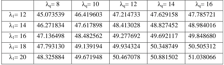
The effect of changes in Demand rate at retailer node and distributor node.

λ_{q= 8} λ_{1= 12 45.073539} λ_{1= 14 46.271834} λ_{1= 16 47.136498} λ_{1= 18 47.793130} λ_{1= 20 48.325884}

Table 2: Total expected cost rate as a function when demand increases

The graph of the demand rate variation is given below and it describes, if the demand rate increases then the total cost also increases.

Figure

144

Total expected cost rate as a function TC(s. Q), s and Q

nalysis

The effect of changes in Demand rate at retailer node and distributor node.

= 8 λ_{q= 10} λ_{q= 12} λ_{q= 14}

45.073539 46.419603 47.214733 47.629158

46.271834 47.617898 48.413028 48.827452

47.136498 48.482562 49.277692 49.692117

47.793130 49.139194 49.934324 50.348749

48.325884 49.671948 50.467078 50.881502

Total expected cost rate as a function when demand increases

The graph of the demand rate variation is given below and it describes, if the demand rate increases then the total cost also increases.

Figure 2: TC(s, Q) for different demand rates

Total expected cost rate as a function TC(s. Q), s and Q

The effect of changes in Demand rate at retailer node and distributor node.

λ_{q= 16}

47.785721 48.984016 49.848680 50.505312 51.038066 Total expected cost rate as a function when demand increases

s=2

S=45 111.998164

S=50 118.699318

S=55 123.090318

S=60 125.576395

S=65 126.984419

Table 3: Total expected cost rate as a function when s and S increases

Figure

From the graph it is identified that the total cost

hD=0.04

hR=0.002 30.8517816

hR=0.004 30.8598022

hR=0.006 30.8678228

hR=0.008 30.8758424

hR=0.010 30.883863

Table 4:

Figure

Backlogging

145

s=4 s=6 s=8

111.998164 118.761642 124.799813 130.664478

118.699318 124.359054 129.299781 133.996082

123.090318 127.562168 131.434202 135.090008

125.576395 129.128145 132.243072 135.192545

126.984419 130.065937 132.851239 135.511516

Total expected cost rate as a function when s and S increases

Figure 3: TC(s, Q) for different s and S values

From the graph it is identified that the total cost increases when the s and S increases.

=0.04 hD=0.08 hD=0.12 hD=0.16

30.8517816 31.3422 31.8325 32.3229

30.8598022 31.3502 31.8405 32.3309

30.8678228 31.3582 31.8486 32.3389

30.8758424 31.3662 31.8566 32.3469

30.883863 31.3742 31.8646 32.355

Total expected cost rate when hR and hD increases

Figure 4: TC(s, Q) for different hR and hD values

s=10 136.843108 138.773110 138.765317 138.137225 138.145444 Total expected cost rate as a function when s and S increases

increases when the s and S increases. hD=0.20

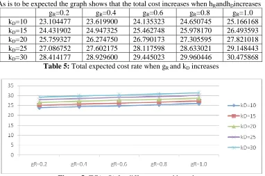
As is to be expected the graph shows that the gR=0.2

kD=10 23.104477

kD=15 24.431902

kD=20 25.759327

kD=25 27.086752

kD=30 28.414177

Table 5:

Figure

6. Conclusion

In this model a three level supply chain consisting of a single product, one manufacturing facility, one Distribution centre (DC) and one retailer.. The model is analyzed within the framework of Markov processes.. Various system performance measures are derived and the long-run expected cost rate is calculated. By assuming a suitable cost structure on the inventory system, we have presented extensive numerical illustrations to show the effect of change of values on the total expected cost rate. It would be interesting to a

problem discussed in this paper by relaxing the assumption of exponentially distributed lead-times to a class of arbitrarily distributed lead

model can be used to generate various special eases.

1. S.Axsater, Exact and approximate evaluation of batch ordering policies inventory systems, Oper. Res.

2. B.M.Beamon, Supply

Journal of Production Economics

3. E.Cinlar, Introduction to Stochastic 'Processes 1975.

4. A.J.Clark and H.Scarf,

Management Science

5. G.Hadley and T.M.Whitin, Cliff. (1963).

6. F.Harris, Operations and costs, f 48-52, (1915).

146

As is to be expected the graph shows that the total cost increases when hR

gR=0.4 gR=0.6 gR=0.8

23.104477 23.619900 24.135323 24.650745

24.431902 24.947325 25.462748 25.978170

25.759327 26.274750 26.790173 27.305595

27.086752 27.602175 28.117598 28.633021

28.414177 28.929600 29.445023 29.960446

Total expected cost rate when gR and kD increases

Figure 5: TC(s, Q) for different gR and kD values

three level supply chain consisting of a single product, one manufacturing facility, one Distribution centre (DC) and one retailer.. The model is analyzed within the framework of Markov processes.. Various system performance measures are derived and run expected cost rate is calculated. By assuming a suitable cost structure on the inventory system, we have presented extensive numerical illustrations to show the effect of change of values on the total expected cost rate. It would be interesting to a

problem discussed in this paper by relaxing the assumption of exponentially distributed times to a class of arbitrarily distributed lead-times. Once this is done, the general model can be used to generate various special eases.

REFERENCES

Axsater, Exact and approximate evaluation of batch ordering policies

Oper. Res., 41 (1993) 777-785.

Supply chain design and analysis: models and methods,

Journal of Production Economics, 55(3) (1998) 281-294.

Introduction to Stochastic 'Processes, Prentice Hall,

Engle-and H.Scarf, Optimal policies for a multi- echelon inventory prob

Management Science, 6(4) (1960) 475-490.

Whitin, Analysis of inventory systems, Prentice-Hall, Englewood

Operations and costs, factory management series, A.W.Shah Co., Chicago,

RandhDincreases

gR=1.0

25.166168 26.493593 27.821018 29.148443 30.475868 increases

three level supply chain consisting of a single product, one manufacturing facility, one Distribution centre (DC) and one retailer.. The model is analyzed within the framework of Markov processes.. Various system performance measures are derived and run expected cost rate is calculated. By assuming a suitable cost structure on the inventory system, we have presented extensive numerical illustrations to show the effect of change of values on the total expected cost rate. It would be interesting to analyze the problem discussed in this paper by relaxing the assumption of exponentially distributed times. Once this is done, the general

Axsater, Exact and approximate evaluation of batch ordering policies for two level

nd analysis: models and methods, International

-wood Cliffs, NJ,

echelon inventory problem,

Hall, Englewood

Backlogging

147

7. S.Kalpakam and G.Arivarigan, A coordinated multicommodity (s, S) inventory system, Mathematical and Computer Modelling, 18 (1993) 69-73.

8. A.Krishnamoorthy, R.I.Basha and B.Lakshmy, Analysis of a two commodity problem, International Journal of Information and Management Sciences, 5(1) (1994) 127-136.

9. A.Krishnamoorthy and T.V.Varghese, A two commodity inventory problem,

International Journal of Information and Management Sciences, 5(3) (1994) 55-70.

10. K.Krishnan, Stochastic Modeling in Supply Chain Management System, unpublished Ph.D., Thesis, Madurai Kamaraj University, Madurai, (2007).

11. J.Medhi, Stochastic processes, Third edition, New Age International Publishers, New Delhi, (2009).

12. E.Naddor, Inventory System, John Wiley and Sons, New York, (1966).

13. S.Nahmias, Perishable inventory theory; a review, Opsearch, 30 (1982) 680-708. 14. S.Nahmias and S.S.Wang, A heuristic lot size reorder point model for decaying

inventories, Management Science, 25 (1979) 90-97.

15. S.Nahmias, On the equivalence of three approximate continuous review models,

Naval Research Logistics Quarterly, 23 (1974) 31 - 36.

16. S.Nahmias, Optimal ordering policies for perishable inventory-II, Operations

Research, 23 (1975) 735 - 749.

17. M.Rameshpandi, C.Periyasamy and K.Krishnan, Analysis of two-echelon perishable inventory system with direct and retrial demands, IOSR Journal of Mathematics, 10 (5) (2014) 51-57.

18. M.Rameshpandi, C.Periyasamy and K.Krishnan, Two Echelon inventory system with finite population and retrial demands, Proceedings of the National conference on Mathematical Modelling, (2014) 128-135.

19. M.Rameshpandi and K.Krishnan, Stochastic analysis of perishable inventory system, Proceedings of the National seminar on Recent Trends in Applied Mathematics (RTAM-2015) (2015) 32-39.

20. B.D.Sivazlian, Stationary analysis of a multi-commodity inventory system with interacting set-up costs, SIAM Journal of Applied Mathematics, 20(2) (1975) 264-278.

21. B.D.Sivazlian and L.E.Stanfel, Analysis of systems in Operations Research, First edition, Prentice Hall, (1974).

22. A.F.Veinott and H.M.Wagner, Computing optimal (s,S) inventory policies,

Management Science, 11 (1965) 525-552.

23. A.F.Veinott, The status of mathematical inventory theory, Management Science, 12 (1966) 745-777.

24. V.S.S.Yadavalli, N.Anbazhagan and G.Arivarignan, A two commodity continuous review inventory system with lost sales, Stochastic Analysis and Applications, 22 (2004) 479-497.

25. V.S.S.Yadavalli, W.C.De and S.Udayabaskaran, A substitutable two-product inventory system with joint ordering policy and common demand, Applied