Fitting Data with Different Error Models »

Fitting Data with Different

Error Models

Béla Paláncz

A maximum likelihood estimator has been applied to find

regression parameters of a straight line in case of different error models. Assuming Gaussian-type noise for the measurement errors, explicit results for the parameters can be given

employing Mathematica. In the case of the ordinary least squares (OLSy), total least squares (TLS), and least geometric mean deviation (LGMD) approaches, as well as the error model of combining ordinary least squares (OLSx and OLSy) in the Pareto sense, simple formulas are given to compute the parameters via a reduced Gröbner basis. Numerical examples illustrate the methods, and the results are checked via direct global minimization of the residuals.

‡

Introduction

Generally, to carry out a regression procedure one needs to have a model MHx,y,qL=0, an error definition e_MHx,y:qL, and the probability density function of the error PDFHe_MHx,y:qLL. Considering the set 8Hx₁,y₁L,Hx₂,y₂L, …,Hxn,ynL< as measurement

points, the maximum likelihood approach aims at finding the parameter vector q that maxi-mizes the likelihood of the joint error distribution. Assuming that the measurement errors are independent, we should maximize (see eg. [1])

(1) PDFHe_MHHx₁,y₁L:qL, e_MHHx₂,y₂L:qL, ...,e_MHHxn,ynL:qLL=

‰ i=1

n

PDFHe_MHHxi,yiL:qLL.

Consider the Gaussian-type error distribution as NH0,sL; then our estimator is

(3) LHqL= -‚

i=1

n

ln e

-eMHHxi,yiL:qL 2

2s2 2p s

=nlnK 2p sO+‚ i=1

n _e

MHHxi,yiL:qL2

2s2 .

In our case the model is a line,

(4) LHm,bLdef= ‚

i=1

n _He

MHHxi,yiL:Hm,bLLL2

2s2 .

It can be seen that (in the case of Gaussian-type measurement noise) only the type of the error model determines the parameter values, since we should always minimize the least squares of the errors. There are different error models, which can be applied to fitting a line in a least-squares sense. The error model frequently employed, assuming an error-free independent variable x, is the ordinary least squares model (OLSy)

(5) e_MHHx,yL:Hm,bLL= y-mx-b.

Similarly, one may also consider an error-free dependent variable y. Then the error model (OLSx) is

(6) e_MHHx,yL:Hm,bLL= x- -b+y

m .

These approaches are called the algebraic approach.

Another error model considers the geometrical distance between the data point and the line to be fitted. This type of fitting is also known as orthogonal regression, since the distances of the sample points from the line are evaluated by computing the orthogonal projection of the measurements on the line itself. The error in this case [2] is

(7) e_MHHx,yL:Hm,bLL= y-m x-b

1+m2

.

This geometrical approach or total least squares (TLS) approach can also be considered as an optimization problem with constraints; namely, one should minimize the errors in both variables [3]:

(8)

‚ i=1

n

Dx_i2+ Dy_i2Ømin

under the conditions

In addition, one can also combine OLSx and OLSy to construct an error model. The first

possibility is to consider the geometric mean of these two types of errors,

(10) e_MHHx,yL:Hm,bLL= H-b-m x+yL x- -b+y

m .

These error models are illustrated in Figure 1.

GraphicsA9

Arrow@88-1, 0<, 810, 0<<D, Arrow@880, -1<, 80, 7<<D, Line@883, 2<, 88, 2<<D, Line@883, 2<, 83, 6<<D,

8Thick, Line@883, 6<-.285, -4<, 88, 2<+.285, -4<<D<, Line@883, 2<, 83, 2<+880ê41, 100ê41<<D,

StyleATextA"OLS"Style@"x",ItalicD, H83, 2<+88, 2<L ê2, 80, 2<E,

16E,

StyleATextA"OLS"Style@"y",ItalicD, H83, 2<+83, 6<L ê2, 81.5, 0<E, 16E,

Style@Text@"TLS", H283, 2<+880ê41, 100ê41<L ê2,

8-1.8, 0<D, 16D, Style@

Text@Row@8Style@"y", ItalicD, " = ", Style@"m", ItalicD, " ", Style@"x", ItalicD, " + ", Style@"b", ItalicD <D,

H83, 6<+88, 2<L ê2, 8-1.5,-1<D, 16D =

OLS

OLS

TLS

y

=

m x

+

b

Ú Figure 1. The different error models in the case of fitting a straight line.

This model is also called the leastgeometric mean deviation approach or LGMD model (see [4)]. As a second possibility, one may consider OLSx and OLSy as competing

func-tions of the parameters and find their Pareto-front representing a set of optimal solufunc-tions for the parameters q. Since this multi-objective problem is convex, the objective can be ex-pressed as a linear combination of these error functions, namely

(11) e_MHHxi,yiL:Hm,bLL= lH-b-m x+yL+H1- lL x

--b+y

m ,

where l is a parameter, 0§ l §1, and the set of optimal solutions of the parameters be-longing to the Pareto-front is q=qHlL. You can choose the value of l depending on your trade-off preference between OLS_x and OLS_y [5].

‡

Application of Symbolic Computation

·

SuperLog

Function

SuperLog@Q_D:=Module@ 8erk<,

Which@

Q===On,

Unprotect@LogD; Clear@LogD;

Log@Product@x_, 8k_. a_, b_<DD:=

Log@Product@Times@erk, xD, 8k, a, b<DD ê. erkØ1; Log@Product@HoldPattern@Times@x__DD, 8k_, a_, b_<DD:=

Simplify@

Map@Sum@Ò, 8k, a, b<D&,

PlusüüMap@Expand@PowerExpand@Log@ÒDDD&, List@xDDD êê.

Sum@u_, w_, 8kk_, aa_, bb_<Dß

u Sum@w, 8kk, aa, bb<D ê; FreeQ@u, kkDãTrueD; Protect@LogD;

Print@"SuperLog is now On."D,

Q===Off,

Unprotect@LogD; Clear@LogD; Protect@LogD; Print@"SuperLog is now Off."D,

True,

Print@"Please use SuperLog@OnD or SuperLog@OffD!"D DD

Let us activate this function.

SuperLog@OnD

SuperLog is now On.

Then this is the ML estimator for Gaussian-type noise.

L= ‰

i=1

n

PDF@NormalDistribution@0,sD, eMiD

‰

i=1

n _‰-IeMMi2 2s2

·

Ordinary Least Squares (

OLS

)

Now let us consider the OLSy problem.

LogLAOLSyE=Log@Lê.eMi Øyi-m xi -bD êêSimplify

- b

2_n

2s2

-1

2 nLog@2D

-1

2 nLog@pD-nLog@sD+

‚

i=1

n

-b m xi s2 +‚

i=1 n -m 2_x i 2

2s2 +‚

i=1

n _{b yi}

s2 +‚ i=1

n _{m xi yi}

s2 +‚ i=1

n

- yi

2

2s2

Here are the necessary conditions for the optimum.

eq1AOLSyE=DALogLAOLSyE, mEã0

‚

i=1

n

-b xi s2 +‚

i=1

n

-m xi

2

s2 +‚ i=1

n _x

i yi

s2 ã0

eq2AOLSyE=DALogLAOLSyE, bEã0

-b n s2 +‚

i=1

n

-m xi s2 +‚

i=1

n _y

i

s2 ã0

Let us introduce the following constants:

(12)

a=‚

i=1

n

x_i,

(13)

b=‚

i=1

n

x_i2,

(14)

c=‚

i=1

n

yi,

(15)

d=‚

i=1

n

y_i2,

(16)

e=‚

i=1

n

In those terms, here are the necessary conditions for the optimum.

Eq1AOLSyE= -ab-bm+eã0

e-ab-bmã0

Eq2AOLSyE= -b n- am+cã0

c-am-b nã0

Then this is the optimal solution of the parameters.

solmbG=SolveA9Eq1AOLSyE, Eq2AOLSyE=, 8m, b<E êêFlatten

:mØ --a c+en

a2_-bn , bØ

-b c-a e

a2_-bn >

·

Total Least Squares (

TLS

)

Although the equation system for the parameters of OLSy is linear, for other error models

we get a multivariable algebraic system. Now consider the TLS problem. Here is the maxi-mum likelihood function.

LogL@TLSD=LogBLê.e_Mi -> yi-m xi -b

1+m2

F êêSimplify

- b

2n

2I1+m2_Ms2

-1

2 nLog@2D

-1

2 nLog@pD-nLog@sD+_i=1‚

n

- b m xi I1+m2_Ms2 +

‚

i=1

n

- m

2x i 2

2I1+m2_Ms2 +‚

i=1

n _{b yi}

I1+m2_Ms2 +‚ i=1

n _{m xi yi}

I1+m2_Ms2 +‚ i=1

n

- yi

2

Therefore here is the equation system to be solved.

eq1@TLSD=D@LogL@TLSD, mDã0êêSimplify

b2_{m n}

I1+m2_M2_s2

+‚

i=1

n _{2b m}2_x i

I1+m2_M2_s2

- b xi

I1+m2_Ms2 +

‚

i=1

n _m3_x

i 2

I1+m2_M2_s2

- m xi

2

I1+m2_Ms2 +‚ i=1

n

- 2b m yi I1+m2_M2_s2

+

‚

i=1

n _{m y}

i 2

I1+m2_M2_s2

+‚

i=1

n

- 2m

2x iyi

I1+m2_M2_s2

+ xi yi

I1+m2_Ms2 ã0

eq2@TLSD=D@LogL@TLSD, bDã0êêSimplify

‚

i=1

n

- m xi

I1+m2_Ms2 +‚ i=1

n _yi

I1+m2_Ms2 ã

b n

I1+m2_Ms2

Since 1+m2_{¹≠0, the conditions are as follows.}

Eq1@TLSD=

b2_{m n+a 2b m}2_-aI1+m2_{Mb+ bm}3_{- bmI1+m}2_{M-2 cb m+} dm-2 em2+eI1+m2Mã0

dm-2 cb m-2 em2+2 ab m2+bm3+

eI1+m2_{M-abI1+m}2_{M-bmI1+m}2_M+b2_{m nã0}

Eq2@TLSD= -b n-am+cã0

c-am-b nã0

A Gröbner basis solves this system, eliminating b.

gbm@TLSD=GroebnerBasis@8Eq1@TLSD, Eq2@TLSD<, 8m, b<, 8b<D êê

Simplify

solm@TLSD=Solve@gbm@TLSDã0,mD êêFlatten

:mØ 1

2Ha c-enL -a

2_+c2_+bn-dn

-Ia2-c2-bn+dnM2-4Ha c-enL H-a c+enL ,

mØ 1

2Ha c-enL -a

2_+c2_{+bn-dn+}

Ia2_-c2_{-bn+dnM}2_{-4Ha c-enL H-a c+enL >}

Since the second equation is linear, it is reasonable to compute m first, then b.

solb@TLSD=Solve@Eq2@TLSD, bD êêFlatten

:bØ c-am

n >

·

Least Geometric Mean Deviation (

LGMD

)

The LGMD error model also leads to a second-order polynomial equation system. Now here is the ML estimator.

LogL@LGMDD=LogBLê.eMiØ H-b-m xi+yiL xi

--b+yi m F êê Simplify

b2n

2ms2

-1

2 nLog@2D

-1

2 nLog@pD-nLog@sD+

‚

i=1

n _{b xi}

s2 +‚ i=1

n _{m x}

i 2

2s2 +‚

i=1

n

- b yi

ms2 +‚

i=1

n

-xiyi s2 +‚

i=1

n _y

i 2

Consequently, here is the system to be solved for the parameters.

eq1@LGMDD=D@LogL@LGMDD, mDã0êêSimplify

‚

i=1

n _x

i 2

2s2 +‚

i=1

n _{b yi}

m2_s2 +‚ i=1

n

- yi

2

2m2_s2 ã

b2n

2m2_s2

eq2@LGMDD=D@LogL@LGMDD, bDã0

b n

ms2 +‚

i=1

n _xi

s2 +‚ i=1

n

- yi

ms2 ã0

Assume m¹≠0.

Eq1@LGMDD= -b2n+m2b+2bc-dã0

-d+2 cb+bm2-b2nã0

Eq2@LGMDD=b n+ma-cã0

-c+am+b nã0

Again a Gröbner basis gives a second-order system.

gbm@LGMDD=

GroebnerBasis@8Eq1@LGMDD, Eq2@LGMDD<,8m, b<, 8b<D êê

Simplify

9c2_-a2_m2_-dn+bm2_n=

solmT=Solve@gbm@LGMDDã0, mD êêFlatten

:mØ - c

2_-dn

a2_-bn

, mØ c

2_-dn

a2_-bn

>

When m is known, the other parameter can be computed.

solbT=Solve@Eq2@LGMDD, bD êêFlatten

:bØ c-am

·

Pareto Approach

In the case of the Pareto approach, the system is already fourth order.

LogL@ParetoD=

LogBLê.:eMiØ lH-b-m xi+yiL2+H1- lL xi

--b+yi m 2 >F êê Simplify - b 2n

2m2_s2

-b2n_l

2s2 +

b2n_l

2m2_s2

-1

2 nLog@2D

-1

2 nLog@pD-nLog@sD+

‚

i=1

n

- b xi

ms2 +‚

i=1

n _blxi

ms2 +‚

i=1

n

-b mlxi s2 +‚

i=1

n

- xi

2

2s2 +‚

i=1

n _lx

i 2

2s2 +

‚

i=1

n

-m

2_lx i 2

2s2 +‚

i=1

n _{b y}

i

m2_s2 +‚ i=1

n _bly

i

s2 +‚ i=1

n

-blyi

m2_s2 +‚ i=1

n _x

i yi

ms2 +

‚

i=1

n

-lxiyi

ms2 +‚

i=1

n _{mlxi yi}

s2 +‚ i=1

n

- yi

2

2m2_s2 +‚

i=1

n

-lyi

2

2s2 +‚

i=1

n _ly

i 2

2m2_s2

Here is the system.

eq1@ParetoD=D@LogL@ParetoD,mDã0êêSimplify

b2_n

m3_s2 +‚ i=1

n _{b x}

i

m2_s2 +‚ i=1

n

-blxi s2 +‚

i=1

n

-blxi

m2_s2 +

‚

i=1

n

-mlxi

2

s2 +‚ i=1

n

-2b yi

m3_s2 +‚ i=1

n _2blyi

m3_s2 +‚

i=1

n

- xi yi

m2_s2 +

‚

i=1

n _{lxi yi}

s2 +‚ i=1

n _lxiyi

m2_s2 +‚

i=1

n _y

i 2

m3_s2 +‚ i=1

n

- lyi

2

m3_s2 ã

b2n_l

m3_s2

eq2@ParetoD=D@LogL@ParetoD,bDã0êêSimplify

b nl

m2_s2 +‚ i=1

n

- xi

ms2 +‚

i=1

n _lxi

ms2 +‚

i=1

n

-mlxi s2 +

Here is the system in compact form.

Eq1@ParetoD=

b2_n-b2_{nl +m ba-m}3_{bla-m bla-m}4_{lb-2bc+2blc} -me+m3le+mle+d-dl ã0

d-2 cb-em+ab m+b2_{n-dl +2 cbl +}

eml -ab ml +em3l -ab m3l -bm4l -b2nl ã0

Eq2@ParetoD=

-b n-m2_{b nl +b nl -ma+mla-m}3 _la+c+m2_{lc- lcã0}

c-am-b n-cl +aml +cm2l -am3l +b nl -b m2_{nl ã0}

Here is the Gröbner basis for the first parameter.

gbm@ParetoD=

GroebnerBasis@8Eq1@ParetoD, Eq2@ParetoD<, 8m, b<, 8b<D êê

Simplify

9I1+I-1+m2MlM Idn-em n+c2H-1+ lL+a2m4l

-dnl +em nl +em3_{nl -bm}4_{nl -a cmI-1+ l +m}2_lMM=

Assume that 1+I-1+m2_Ml¹≠0.

Gbm=dn-em n+c2H-1+ lL+a2m4l -dnl +em nl +em3nl

-bm4nl -a cmI-1+ l +m2lM êêExpand

-c2+a cm+dn-em n+c2l -a cml

-a cm3l +a2m4l -dnl +em nl +em3nl -bm4nl

After solving this polynomial for m, the other parameter can be solved from the second equation, which is linear in b.

solbP=Solve@Eq2@ParetoD, bD êêFlatten

:bØ c-am

‡

Numerical Example

·

Data Samples

Consider some data on rainfall x (in mm) and the resulting groundwater level changes y (in cm) from a landslide along the Ohio River Valley near Cincinnati, Ohio [7].

xydata=881.94, 2.5<, 83.33, 1.89<, 83.22, 1.67<,

85.67, 1.31<, 84.72, 1.02<, 83.89, 0.96<, 82.78, 1.1<,

810.56, 0.15<, 89.44, 3.92<, 812.78, 5.23<,

814.72, 4.22<, 813.61, 3.63<, 820.39, 4.32<,

838.89, 5.89<<;

There are 14 measurements.

Length@xydataD

14

This displays the measured data.

ListPlot@xydata, AxesLabelØ8"x@mmD", "y@cmD"<,

PlotStyleØ[email protected], PlotRangeØ880, 40<, 80, 7<<D

0 10 20 30 40 x@mmD

0 1 2 3 4 5 6 7

y@cmD

·

Computation of the Constants for the Equation Systems

The constants a, b, c, d, and e in equations (12) to (16) are needed.

This separates the data.

8xdata, ydata<=Transpose@xydataD;

This transforms the data into dimensionless form.

xS=Hxdata-Min@xdataDL ê HMax@xdataD-Min@xdataDL; yS=Hydata-Min@ydataDL ê HMax@ydataD-Min@ydataDL;

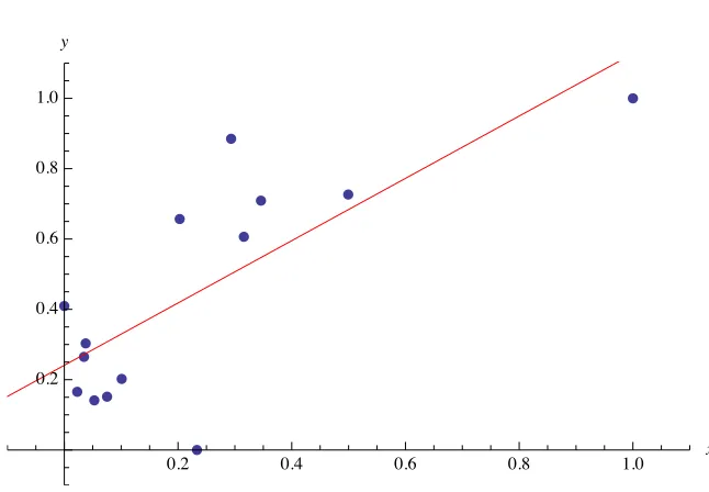
p2=ListPlot@Transpose@8xS, yS<D, AxesLabelØ8x, y<, PlotStyleØ[email protected],

PlotRangeØ88-0.1, 1.1<, 8-0.1, 1.1<<D

0.2 0.4 0.6 0.8 1.0 x

0.2 0.4 0.6 0.8 1.0

y

Ú Figure 3. The measured data: rainfall versus water level change in dimensionless form.

Now the constants can be computed.

abcden=

Join@

Thread@8a, b, c, d, e<Ø

Totalêü8xS, xS ^ 2, yS, yS ^ 2, xS yS<D, 8nØLength@xydataD< D

8aØ3.21461, bØ1.67216,

·

Computation of the Parameters of the Fitted Line

ü OLSy Model

Here are the estimated parameters employing the explicit solutions.

solmbGê. abcden

8mØ0.885963, bØ0.240945<

This checks the result.

Fit@Transpose@8xS, yS<D, 81, t<, tD

0.240945+0.885963 t

Figure 4 shows the estimated line with the sample points.

p3=Plot@%, 8t, -0.1, 1.1<, PlotStyleØRedD;

Show@8p2, p3<D

0.2 0.4 0.6 0.8 1.0 x

0.2 0.4 0.6 0.8 1.0

y

ü TLS Model

Here are the first and second parameters.

solm@TLSD ê. abcden

8mØ1.23716, mØ -0.808306<

solb@TLSD ê. solm@TLSD ê. abcden

8bØ0.160305<

Here is a check of this result on the basis of the TLS definition. Equation (8) gives the ob-jective function.

obj@TLSD=TotalATableADxi2+ Dyi2, 8i, Length@xydataD<EE

Dx₁2+ Dx₂2+ Dx₃2+ Dx₄2+ Dx₅2+ Dx₆2+ Dx₇2+ Dx₈2+ Dx₉2+ Dx₁₀2 _{+ Dx}

11 2 _{+ Dx}

12 2 _{+ Dx}

13 2 _{+ Dx}

14 2 _{+ Dy}

1 2_{+ Dy}

2 2_{+ Dy}

3 2_{+ Dy}

4 2₊

Dy₅2+ Dy₆2+ Dy₇2+ Dy₈2+ Dy₉2+ Dy₁₀2 + Dy₁₁2 + Dy₁₂2 + Dy₁₃2 + Dy₁₄2

The constraints are yi+ Dyi-mHxi+ DxiL-b=0,i=1, …,n.

Hcons=Table@yS@@iDD+ Dy_i-mHxS@@iDD + DxiL-bã0,

8i, Length@xydataD<DL êêColumn

0.409408-b-mH0.+ Dx1L+ Dy1ã0

0.303136-b-mH0.0376184+ Dx2L+ Dy2ã0

0.264808-b-mH0.0346414+ Dx3L+ Dy3ã0

0.202091-b-mH0.100947+ Dx4L+ Dy4 ã0

0.151568-b-mH0.0752368+ Dx5L+ Dy5ã0

0.141115-b-mH0.052774+ Dx6L+ Dy6 ã0

0.165505-b-mH0.0227334+ Dx7L+ Dy7ã0

0.-b-mH0.233288+ Dx8L+ Dy8ã0

0.656794-b-mH0.202977+ Dx9L+ Dy9 ã0

0.885017-b-mH0.293369+ Dx10L+ Dy10ã0

0.709059-b-mH0.345873+ Dx11L+ Dy11ã0

0.606272-b-mH0.315832+ Dx12L+ Dy12ã0

0.726481-b-mH0.499323+ Dx13L+ Dy13ã0

The unknown variables are not only the parameters, but the adjustments HDxi,DyiL as well.

vars=Join@Table@8Dxi,Dyi<, 8i, Length@xydataD<D, 8m,b<D êê Flatten

8Dx1, Dy1, Dx2, Dy2, Dx3, Dy3, Dx4, Dy4, Dx5, Dy5,

Dx6, Dy6, Dx7, Dy7, Dx8, Dy8, Dx9, Dy9, Dx10, Dy10,

Dx11, Dy11, Dx12, Dy12,Dx13, Dy13, Dx14, Dy14, m, b<

This uses a built-in global optimization method. (This takes a long time to compute.)

Timing@

sol=NMinimize@8obj@TLSD, cons<, vars,

MethodØ8"RandomSearch", "SearchPoints"Ø200<D;D

8257.582130, Null<

Drop@sol@@2DD, 81, 2 Length@xydataD<D

8mØ1.23716, bØ0.160305<

The TLS estimation gives a result quite different from the OLSy model; see Figure 5.

p4=Plot@mt+bê.%, 8t, -0.1, 1.1<, PlotStyleØGreenD;

Show@8p2, p3, p4<D

0.2 0.4 0.6 0.8 1.0 x

0.2 0.4 0.6 0.8 1.0

ü LGMD Model

Now here is the first parameter.

solmTê. abcdenêêChop

8mØ -1.17471, mØ1.17471<

This uses the result.

solbTê. solmT@@2DD ê. abcdenêêChop

8bØ0.174644<

Here is a numerical check of the objective.

obj@LGMDD=

TotalB

TableB. H-b-mxS@@iDD+yS@@iDDL2 _xS@@iDD-yS@@iDD-b m

2 ,

8i, Length@xydataD<FF;

solT=NMinimize@obj@LGMDD, 8m, b<D

80.5394, 8mØ1.17471, bØ0.174644<<

Figure 6 shows this result together with the OLSy and TLS models.

Show@8p2, p3, p4, p5<D

0.2 0.4 0.6 0.8 1.0 x

0.2 0.4 0.6 0.8 1.0

y

Ú Figure 6. The lines estimated with the OLSy (red), TLS (green), and LGMD (blue) models.

ü Pareto Approach

The first parameter is a fourth-order polynomial.

Gbmê. abcden

18.0448-11.5853m-18.0448l +

11.5853ml +11.5853m3_{l -13.0765m}4_l

The best trade-off between OLSy and OLSx is to let l =0.5.

solP=NSolve@Gbmê. abcdenê.l Ø1ê2, mD

88mØ -1.0602<, 8mØ0.404042-0.99016Â<,

8mØ0.404042+0.99016Â<, 8mØ1.13808<<

This is the real positive solution.

Using this value gives the second parameter.

solbPê. solP@@4DD ê. abcdenêêFlatten

8bØ0.183054<

We compute the solution using direct global minimization. Here is the objective.

obj@ParetoD=

TotalB

TableB

lH-b-mxS@@iDD+yS@@iDDL2+

H1- lL xS@@iDD-yS@@iDD-b

m

2

,8i, Length@xydataD<FF;

This gives the result.

solP=NMinimize@8obj@ParetoD ê.l Ø1ê2<, 8m, b<, MethodØ8"RandomSearch", "SearchPoints"Ø200<D

80.545029, 8mØ1.13808, bØ0.183054<<

Figure 7 shows this solution with the results of the other models.

Show@8p2, p3, p4, p5, p6<D

0.2 0.4 0.6 0.8 1.0 x

0.2 0.4 0.6 0.8 1.0

y

Ú Figure 7. The lines estimated with the OLSy (red), TLS (green), and LGMD (blue) models, and the

Pareto approach with l =1ê2 (magenta).

‡

Conclusion

The numerical computations show that the formulas developed by an ML estimator via symbolic computation to determine the parameters of a straight line to be fitted provide correct results and require considerably less computation time than the direct methods based on global minimization of the residuals. Our examples also illustrate that the TLS, LGMD, and Pareto approaches give more realistic solutions than the traditional OLSy,

since Figure 7 shows there are at least two outliers in the sample set.

‡

References

[1] W. H. Press, S. A. Teukolsky, W. T. Vetterling, and B. P. Flannery, Numerical Recipes in C, 2nd ed., Cambridge: Cambridge University Press, 1992.

[2] M. Zuliani. “RANSAC for Dummies.” (Jan 10, 2014)

vision.ece.ucsb.edu/~zuliani/Research/RANSAC/docs/RANSAC4Dummies.pdf.

[5] B. Paláncz and J. L. Awange, “Application of Pareto Optimality to Linear Models with Errors-in-All-Variables,” Journal of Geodesy, 86(7),2012 pp. 531–545.

doi:10.1007/s00190-011-0536-1.

[6] C. Rose and M. D. Smith, “Symbolic Maximum Likelihood Estimation with Mathematica,” The Statistician, 49(2), 2000 pp. 229–240. www.jstor.org/stable/2680972.

[7] W. C. Haneberg, Computational Geosciences with Mathematica, Berlin: Springer, 2004.

B. Paláncz, “Fitting Data with Different Error Models,” The Mathematica Journal, 2014. dx.doi.org/doi:10.3888/tmj.16-4.

About the Author

Béla Paláncz received his D.Sc. degree in 1993 from the Hungarian Academy of Sciences and has wide-ranging experience in teaching and research (RWTH Aachen, Imperial Col-lege London, DLR Köln, and Wolfram Research). His main research fields are mathemati-cal modeling and symbolic-numeric computation.

Béla Paláncz

Department of Photogrammetry and Geoinformatics, Budapest University of Technology and Economics 1521 Budapest, Hungary