SEE THROUGH APPROACH FOR THE SOLUTION TO
NODE MOBILITY ISSUE IN UNDERWATER SENSOR
NETWORK (UWSN)
Nishit Walter, Nitin Rakesh CSE Department Amity University, Uttar Pradesh
Sec- 125, Noida, India
ABSTRACT
The top notch problem that we are facing in the field of Underwater Sensor network (UWSN) is of node mobility issue. This well versed problem arise when there is significant deviation in the location of the nodes i.e. from their point of origin to their final position, considering the fact that these nodes are mobile in nature. To tackle this problem we already proposed an approach named SEE THROUGH and this is the continuation of that work as SEE THROUGH approach part 2. The objective of this paper is to make the approach understandable more easily by considering various cases and presenting a dry run for the same Keywords: UWSN; mobility issue; propagation delay; round trip time; network throughput.
INTRODUCTION
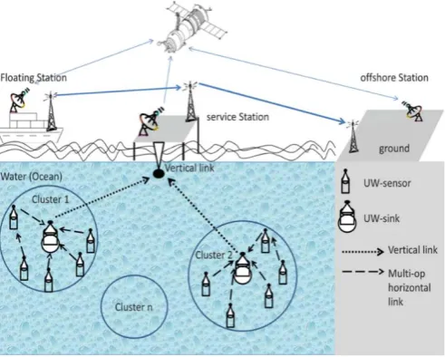
A large number of sensing nodes forming a group are connected to anchors. By making use of Acoustic links the sensing nodes gets connected with one or more underwater sinks.[1-2] Receiving of information and passing of information is done by these sinks to the stations that are on the surface. The formation the sinks employ two kinds of transceivers namely Horizontal Transceiver and Vertical Transceiver. Vertical Transceiver come in handy when the area of application is for long range [3], while on the other hand Horizontal Transceiver are used for the communication between underwater sinks and the sensing nodes.
Stations that are affixed on the surface are also equipped with transceivers for managing a number of communication lines coming from underwater sinks and are also fitted with transmitters so that a communication can be made with the satellite. Information is directly conveyed to these underwater sinks. As the area covered by the communication network is very large, these are not very efficient in terms of energy consumption. [4-7]
The situation of node mobility arise when there is significant deviation in the location of the nodes i.e. from their point of origin to their final position due to the influence of any external activity, be it environmental or manmade.[8-10]
Considering underwater sensor network in terms of 2-D representation [11], facing the problem caused by node mobility, specifically when dealing with the source node and the destination node we have proposed an approach in lieu for its solution, where the communication networks won’t get affected when it comes to node mobility issue and the network can run without causing any lag of failure.
Fig. 2. General depiction of network
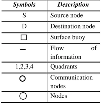
Table for symbols used
Symbols Description
Surface buoy
S Source node
D Destination
node
CN Communication
Considering source node is fixed in quadrant 1 and the destination node is fixed in quadrant 4, there can be 9 ways in which node mobility can occur in regard with source and destination communication:
Fig. 3.1. S moves to Q2 & D moves to Q3
Fig. 3.2. S moves to Q2 & D moves to Q2
Fig. 3.3. S moves to Q2 & D moves to Q1
Fig. 3.5. S moves to Q3 & D moves to Q2
Fig. 3.6. S moves to Q3 & D moves to Q1
Fig. 3.7. S moves to Q4 & D moves to Q3
Fig. 3.8. S moves to Q4 & D moves to Q2
PROPOSED APPROACH
We will be using surface buoys for the solution of node mobility issue.
Fig. 4 sensing nodes and surface buoys
Here, the triangle represents the surface buoys and circles represents the sensing nodes. Both the surface node and the destination node quadrants have knowledge about the communication nodes i.e. source and destination node among which communication is taking place and also about the quadrant to which they belong. Information that is to be relayed from source node to the destination node is made available on the network that is formed by routing protocols.
PROPOSED ALGORITHM FLOWCHART
Fig. 5. Flowchart of proposed approach
DRY RUN OF VARIOUS CASES
We will consider 9 cases where S and D nodes both move simultaneously.
Table for symbols used
Symbols Description
S Source node
D Destination node
Surface buoy
Flow of
information 1,2,3,4 Quadrants
Communication nodes
We are considering information is already present on the network
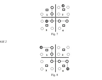
CASE 1
Fig. 6
S moves to quad 2 and D moves to quad 3. This new information is updated to all with the help of surface buoys and the communication node nearest to the destination node relays the information to it as shown in Fig. 7.
Fig. 7
CASE 2
Fig. 8
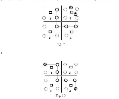
Fig. 9
CASE 3
Fig. 10
S move to quad 2 and D moves to quad 1. As it is clearly visible that quad 1 communication node is closet to D, therefore the data will be transferred to D from that particular node as shown in Fig. 11.
CASE 4
Fig. 12
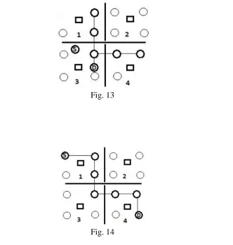
S moves to quad 3 and D moves to quad 3 as well. Communication node of quad 3 is nearest to D, so data will be transferred to D from that node as shown in Fig. 13.
Fig. 13
CASE 5
Fig. 14
Fig. 15
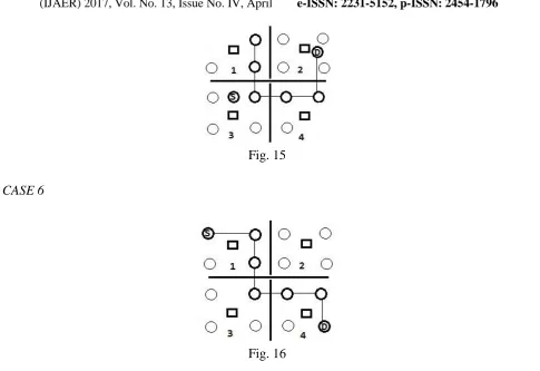
CASE 6
Fig. 16
S moves to quad 3 and D moves to quad 1. Communication node from quad 1 is nearest to D, so data will be transferred to D from that node as shown in Fig. 17.
CASE 7
Fig. 18
S moves to quad 4 and D moves to quad 3. Communication node from quad 3 is nearest to D, so data will be transferred to D from that node as shown in Fig. 19.
Fig. 19
CASE 8
Fig. 20
Fig. 21
CASE 9
Fig. 22
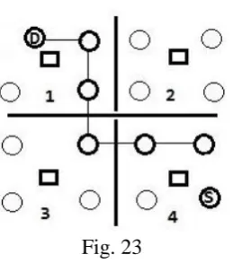
S moves to quad 4 and D moves to quad 1. Communication node from quad 1 is nearest to D, so data will be transferred to D from that node as shown in Fig. 23.
Fig. 23
To calculate network throughput, we are assuming some factors as mentioned below and ideal network conditions means transmission delay, queuing delay, processing delay, transmission delay acknowledgement are considered to be 0, in order to show the difference between ideal case and node mobility cases after applying our proposed algorithm:
Data= 10mb
For ideal case when S is in Q1 & D in 4
Total Distance= 60m Propagation delay= D/S
=60/10 =6s
RTT= 2*propagation delay =2*6
=12s
Network throughput= Size/Time =10mb/12s =.83mb/s
For CASE 1
Total Distance= 30m Propagation delay= D/S
=30/10 =3s
RTT= 2*propagation delay =2*3
=6s
Network throughput= Size/Time =10mb/6s =1.66mb/s
For CASE 2
Total Distance= 50m Propagation delay= D/S
=50/10 =5s
RTT= 2*propagation delay =2*5
=10s
Network throughput= Size/Time =10mb/10s =1mb/s
For CASE 3
Total Distance= 20m Propagation delay= D/S
=2s
RTT= 2*propagation delay =2*2
=4s
Network throughput= Size/Time =10mb/4s =2.5mb/s
For CASE 4
Total Distance= 30m Propagation delay= D/S
=30/10 =3s
RTT= 2*propagation delay =2*3
=6s
Network throughput= Size/Time =10mb/6s =1.66mb/s
For CASE 5
Total Distance= 50m Propagation delay= D/S
=50/10 =5s
RTT= 2*propagation delay =2*5
=10s
Network throughput= Size/Time =10mb/10s =1mb/s
For CASE 6
Total Distance= 10m Propagation delay= D/S
=10/10 =1s
RTT= 2*propagation delay =2*1
=2s
=10mb/2s =5mb/s
For CASE 7
Total Distance= 30m Propagation delay= D/S
=30/10 =3s
RTT= 2*propagation delay =2*3
=6s
Network throughput= Size/Time =10mb/6s =1.66mb/s
For CASE 8
Total Distance= 50m Propagation delay= D/S
=50/10 =5s
RTT= 2*propagation delay =2*5
=10s
Network throughput= Size/Time =10mb/10s =1mb/s
For CASE 9
Total Distance= 10m Propagation delay= D/S
=10/10 =1s
RTT= 2*propagation delay =2*1
=2s
Table for Propagation Delay
Graph 1. Propagation delay of ideal case vs node mobility cases
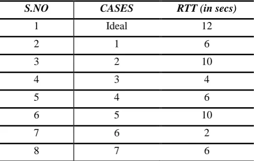
Table IV. Table for round trip time 0 1 2 3 4 5 6 7
1 2 3 4 5 6 7 8 9
Propagation Delay
ideal cases
S.NO CASES PROPAGATION DELAY (in secs)
1 Ideal 6
2 1 3
3 2 5
4 3 2
5 4 3
6 5 5
7 6 1
8 7 3
9 8 5
10 9 1
S.NO CASES RTT (in secs)
1 Ideal 12
2 1 6
3 2 10
4 3 4
5 4 6
6 5 10
7 6 2
Graph 2. Round trip time of ideal case vs node mobility cases
Table V. Table for Network Throughput
S.NO CASES Network Throughput (in mb/s)
1 Ideal .83
2 1 1.66
3 2 1
4 3 2.5
5 4 1.66
6 5 1
7 6 5
8 7 1.66
9 8 1
10 9 5
0 2 4 6 8 10 12 14
1 2 3 4 5 6 7 8 9
RTT
ideal cases
9 8 10
Graph 3. Network Throughput of ideal case vs node mobility cases
Average Network Throughput:
Avg= (1.66+1+2.5+1.66+1+5+1.66+1+5)/9 = 20.48/9
=2.27
Average network throughput of node mobility cases is 2.27mb/s
Graph 4. Graph showing average Network Throughput 0
1 2 3 4 5 6
1 2 3 4 5 6 7 8 9
Network Throughput
ideal cases
0 1 2 3 4 5 6
1 2 3 4 5 6 7 8 9
Avg Network Throughput
Table VI. Table for difference of Network Throughput between ideal and node mobility cases
Graph 5. Graph for showing increament in Network Throughput
Average Increment:
Avg= (.83+.17+1.67+.83+.17+4.17+.83+.17+4.17)/9 =13.01/9
=1.44mb/s
Average increment in Network Throughput of node mobility cases is 1.44mb/s 0
0.5 1 1.5 2 2.5 3 3.5 4 4.5
1 2 3 4 5 6 7 8 9
↑ in Network Throughput
cases
CASES Increase in network Throughput (mb/s)
1 1.66-.83=.83
2 1-.83 =.17
3 2.5-.83 =1.67
4 1.66-.83=.83
5 1-.83 =.17
6 5-.83 =4.17
7 1.66-.83=.83
8 1-.83 =.17
Graph 6. Increament in Network Throughput v/s average Network Throughput
Hence, we have mathematically shown that using our approach we can not only prevent network from failure but also increase the network throughput as shown in the above mentioned graphs.
RESULTS & CONCLUSIONS
We have successfully shown different cases of node mobility issue for source and destination node. Also we have shown as to how communication will resume back to normal in case mobility has taken place among the nodes. In accordance with the previous paper, this paper makes the approach more easily understandable with the help of various cases explained thoroughly in this paper. Second phase of the work i.e. considering various cases of issues have also been worked upon and are explained using graphical as well as tabular form.
FUTURE WORK
In future we can expand our work by simulating the same on some simulating tool or creating real life scenario for the implementation of the work.
REFERENCES
[1] ChinnaDurai, M; MohanKumar, S; Sharmila, “Underwater wireless sensor networks”, Compusoft journal, volume- IV, ISSUE- VII, 1899-1902, 2015
[2] Jan Erik Faugstadmo ; Subsea, Kongsberg Maritime, Horten, Norway ; Magne Pettersen ; Jens M. Hovem ; Arne Lie, “Underwater wireless sensor network”, IEE, 422-427, 2010
[3] J. Heidemann ; Inst. of Inf. Sci., Southern California Univ., CA ; Wei Ye ; J. Wills ; A. Syed, “ Research challenges and applications for underwater sensor networking, IEEE, 228-235, 2006
0 0.5 1 1.5 2 2.5 3 3.5 4 4.5
1 2 3 4 5 6 7 8 9
↑ Network Throughput v/s
Avg
[4] Ian F. Akylidiz, Dario Pompili, Tommaso Melodia, “Challenges For Efficient Communication in Underwater Acoustic Sensor Network”, ACM, 2004.
[5] U.Devee Prasan and Dr. S. Murugappan, “Underwater Sensor Networks: Architecture, Research Challenges and Potential Applications” International Journal of Engineering Research and Applications, Vol. 2, Issue 2, pp.251-256, Mar-Apr 2012.
[6] Jun-Hong Cui ; Connecticut Univ., Storrs, CT, USA ; Jiejun Kong ; M. Gerla ; Shengli Zhou, “ The challenges of building mobile underwater wireless ntworks for aquatic applications”, IEEE, vol 20, issue 3, 12-18, 2006
[7] Jim Partan, Jim Kurose, Brian Neil Levine, “ A survey of practical issues in underwater networks”, ACM, VOL-11, ISSUE-4, 23-33, 2007
[8] Djauhari, M., & Gan, S. Optimality problem of network topology in stocks market analysis. Physica A: Statistical Mechanics and Its Applications, 419, 108-114, 2015
[9] Dario Pompili, Rutgers and Ian F. Akyildiz, “Overview of Networking Protocols for Underwater Wireless Communications”, IEEE Communications Magazine, January, pp 97-102, 2009.
[10] Mohamed K. Watfa, Tala Nsouli, Maya Al-Ayache and Omar Ayyash “Reactive localization in underwater wireless sensor Networks”, University of Wollongong in Dubai – Papers, 2010.
[11] Nishit Walter, Nitin Rakesh “SEE THROUGH approach for the solution to node mobility issue in underwater sensor network (UWSN)” SSIC 2017, SPRINGER 2017, accepted in press.
[12] S. Naik and Manisha J. Nene, “Realization of 3d underwater wireless sensor networks and influence of ocean parameters on node location estimation”, International Journal of Wireless & Mobile Networks (IJWMN) Vol. 4, No. 2, April 2012.
[13] Nishit Walter, Nitin Rakesh “KRUSH-D approach for the solution to node mobility issue in Underwater sensor network (UWSN)”, International Conference on Recent Advancements in Computer Communication and Computational Sciences (ICRAC3S-2016), Springer 2016, ,
accepted, in press.
[14] Kanika Agarwal, Nitin Rakesh “Node Mobility Issues in Underwater Wireless Sensor Network”, International Conference on Computer, Communication, and Computational Sciences (IC4S-2016), Springer 2016, accepted, in press.