https://doi.org/10.5194/gmd-12-2155-2019 © Author(s) 2019. This work is distributed under the Creative Commons Attribution 4.0 License.
The Monash Simple Climate Model experiments (MSCM-DB v1.0):
an interactive database of mean climate, climate change, and
scenario simulations
Dietmar Dommenget1, Kerry Nice1,4, Tobias Bayr2, Dieter Kasang3, Christian Stassen1, and Michael Rezny1
1Monash University, School of Earth, Atmosphere and Environment, Clayton, Victoria 3800, Australia 2GEMOAR Helmholtz Centre for Ocean Research, Düsternbrooker Weg 20, 24105 Kiel, Germany 3DKRZ, Hamburg, Germany
4Transport, Health, and Urban Design Hub, Faculty of Architecture, Building, and Planning, University of Melbourne,
Victoria 3010, Australia
Correspondence:Dietmar Dommenget ([email protected]) Received: 12 June 2018 – Discussion started: 1 August 2018
Revised: 11 April 2019 – Accepted: 26 April 2019 – Published: 3 June 2019
Abstract.This study introduces the Monash Simple Climate Model (MSCM) experiment database. The simulations are based on the Globally Resolved Energy Balance (GREB) model to study three different aspects of climate model sim-ulations: (1) understanding processes that control the mean climate, (2) the response of the climate to a doubling of the CO2concentration, and (3) scenarios of external forcing
(CO2 concentration and solar radiation). A series of
sensi-tivity experiments in which elements of the climate system are turned off in various combinations are used to address (1) and (2). This database currently provides more than 1300 experiments and has an online web interface for fast anal-ysis and free access to the data. We briefly outline the de-sign of all experiments, give a discussion of some results, put the findings into the context of previously published re-sults from similar experiments, discuss the quality and limi-tations of the MSCM experiments, and also give an outlook on possible further developments. The GREB model simula-tion is quite realistic, but the model without flux correcsimula-tions has a root mean square error in the mean state of the sur-face temperature of about 10◦C, which is larger than those of general circulation models (2◦C). It needs to be noted here that the GREB model does not simulate circulation changes or changes in cloud cover (feedbacks). However, the MSCM experiments show good agreement to previously published studies. Although GREB is a very simple model, it delivers good first-order estimates, is very fast, highly accessible, and can be used to quickly try many different sensitivity
exper-iments or scenarios. It builds a basis on which conceptual ideas can be tested to first order and it provides a null hy-pothesis for understanding complex climate interactions in the context of response to external forcing or interactions in the climate subsystems.
1 Introduction
Our understanding of the dynamics of the climate system and climate changes is strongly linked to the analysis of model simulations of the climate system using a range of climate models that vary in complexity and sophistication. Climate model simulations help us to predict future climate changes and they help us to gain a better understanding of the dynam-ics of this complex system.
complex models. They also help in understanding interac-tions in the complex system.
In this article, we introduce the Monash Simple Climate Model (MSCM) database (version: MSCM-DB v1.0). The MSCM is an interactive website (http://mscm.dkrz.de for Germany, last access: 22 May 2018; and http://monash.edu/ research/simple-climate-model for Australia, last access: 22 May 2018) and database that provides access to a series of more than 1300 experiments with the Globally Resolved En-ergy Balance (GREB) model (Dommenget and Floter, 2011; hereafter referred to as DF11). The GREB model was primar-ily developed to conceptually understand the physical pro-cesses that control the global warming pattern in response to an increase in CO2concentration. It therefore centres around
the surface temperature (Tsurf)tendency equation and only
simulates the processes and variables needed for resolving the global warming pattern.
Simplified climate models, such as Earth system models of intermediate complexity (EMICs), often aim at reduc-ing the complexity to increase computation speed and there-fore allow for faster model simulations (e.g. CLIMBER – Petoukhov et al., 2000; UVic – Weaver et al., 2001; FA-MOUS – Smith et al., 2008; LOVECLIM – Goosse et al., 2010). These EMICs are very similar in structure to state-of-the-art coupled general circulation models (CGCMs), fol-lowing the approach of simulating geophysical fluid dynam-ics. The GREB model differs in that it follows an energy bal-ance approach and does not simulate the geophysical fluid dynamics of the atmosphere. It is therefore a climate model that does not include weather dynamics but focusses on the long-term mean climate and its response to external bound-ary changes. It also does not include cloud feedbacks or ad-justments in the atmospheric circulation, as both are given as boundary conditions. However, it does include the most im-portant water vapour, black-body radiation, and ice–albedo feedbacks.
The purposes of the MSCM database for research studies are the following.
– First guess: The MSCM provides first guesses for how the climate may change in idealized or realistic experi-ments. The MSCM experiments can be used to test ideas before implementing and testing them in more detailed CGCM simulations.
– Null hypothesis: The simplicity of the GREB model provides a good null hypothesis for understanding the climate system. Because it does not simulate weather dynamics or circulation changes on a large or small scale, it provides the null hypothesis of a climate as a pure energy balance problem.
– Conceptual understanding: The simplicity of the GREB model helps us to better understand the interactions in the complex climate and therefore helps to formulate simple conceptual models for climate interactions.
– Education: Studying the results of the MSCM helps us to understand the interactions that control the mean state of the climate and its regional and seasonal differences. It helps us to understand how the climate will respond to external forcings in a first-order approximation. The MSCM provides interfaces for fast analysis of experi-ments and selection of data (see Figs. 1–3). It is designed for teaching and outreach purposes but also provides a use-ful tool for researchers. The focus in this study will be on describing the research aspects of the MSCM, whereas the teaching aspects of it will not be discussed. The MSCM ex-periments focus on three different aspects of climate model simulations: (1) understanding the processes that control the mean climate, (2) the response of the climate to a doubling of the CO2concentration, and (3) scenarios of external CO2
concentration and solar radiation forcings. We will provide a short outline of the design of all experiments, give a brief dis-cussion of some results, and put the findings into the context of previously published literature results from similar exper-iments.
The DF11 study focussed primarily on the development of the model equations and a discussion of the response pattern to an increase in CO2 concentration. This study will give a
more detailed discussion on the performance of the GREB model in simulations of the mean state of the climate and a wider range of external forcing scenarios, including solar radiation changes.
The paper is organized as follows: the following sec-tion describes the GREB model, the experiment designs, the MSCM interface, and the input data used. A short analysis of the experiments is given in Sect. 3. This section will mostly focus on the GREB model performance in comparison to ob-servations and previously published simulations in the liter-ature, but it will also give some indications of the findings in the model experiments and the limitations of the GREB model. The final section will give a short summary and out-look for potential future developments and analysis.
2 Model and experiment descriptions
The GREB model is the underlying modelling tool for the MSCM interface. The development of the model and all equations have been presented in DF11. The model is sim-ulating the global climate on a horizontal grid of 3.75◦ lon-gitude×3.75◦ latitude and in three vertical layers: surface, atmosphere, and subsurface ocean. It simulates four prog-nostic variables: surface, atmospheric and subsurface ocean temperature, and atmospheric humidity (column-integrated water vapour); see Appendix Eqs. (A1)–(A4). It further sim-ulates a number of diagnostic variables, such as precipita-tion and snow–ice cover, resulting from the simulaprecipita-tion of the prognostic variables.
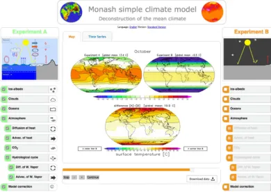
Figure 1.MSCM interface running the deconstruction of the mean climate experiments. Experiment A, on the left, has all processes turned ON, and experiment B, on the right, has all turned OFF. TheTsurfof experiment A is shown in the upper left map, experiment B in the upper
right, and the difference between the two in the lower map. The example shows the values for the October mean.
thermal (long-wave) radiation, the hydrological cycle (in-cluding evaporation, moisture transport, and precipitation), horizontal transport of heat, and heat uptake in the subsurface ocean. Atmospheric circulation and cloud cover are season-ally prescribed boundary conditions, and state-independent flux corrections are used to keep the GREB model close to the observed mean climate. Thus, the GREB model does not simulate the atmospheric or ocean circulation and is there-fore conceptually very different from CGCM simulations.
The model simulates important climate feedbacks, such as the water vapour and ice–albedo feedback, but an important limitation of the GREB model is that the response to exter-nal forcings or model parameter perturbations does not in-volve circulation or cloud feedbacks (Bony et al., 2006, 2015; Boucher et al., 2013). Circulation and cloud feedbacks alter the climate response to external forcings on a regional and, to a lesser extent, global scale. The experiments of this database neglect any effects resulting from cloud or circulation feed-backs. These experiments should therefore only be consid-ered as first-guess estimates. In the context of some of the results discussed further below we will point out some of the limitations of the GREB model approach.
Input climatologies (e.g. Tsurf or atmospheric humidity)
for the GREB model are taken from National Centers for Environmental Protection (NCEP) reanalysis data for 1950–
2008 (Kalnay et al., 1996), cloud cover climatology from the International Satellite Cloud Climatology Project (IS-CCP) (Rossow and Schiffer, 1991), ocean mixed layer depth climatology from Lorbacher et al. (2006), and topographic data from the ECHAM5 atmosphere model (Roeckner et al., 2003).
GREB does not have any internal (natural) variability since daily weather systems are not simulated. Subsequently, the control climate or response to external forcings can be es-timated from one single year. The primary advantages of the GREB model in the context of this study are its simplicity, speed, and low computational cost. A 1-year GREB model simulation can be done on a standard personal computer in about 1 s (about 100 000 simulated years per day). It can do simulations of the global climate much faster than any state-of-the-art climate model and is therefore a good first-guess approach to test ideas before they are applied to more com-plex CGCMs. A further advantage is the lag of internal vari-ability, which allows for the detection of a response to exter-nal forcing much more easily.
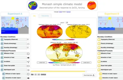
Figure 2.MSCM interface running the deconstruction of the response to a doubling of the CO2concentration in experiments. Experiment
A, on the left, has all processes turned ON, and experiment B, on the right, has all turned OFF. TheTsurfresponse of experiment A is shown
in the upper left map, experiment B in the upper right, and the difference between the two in the lower map. The example shows the annual mean values after 28 years.
(switches; see Fig. 1). For each of these switches, a term in the model equations is set to zero or altered if the switch is OFF. The processes and how they affect the model equa-tions are briefly listed below (with a short summary in Ta-ble 1). The model equations relevant for the experiments in this study are briefly restated in Appendix A1 for the purpose of explaining each experimental set-up in the MSCM.
Ice albedo. The surface albedo (αsurf)and the heat capacity
over ocean points (γsurf)are influenced by snow and sea ice
cover. In the GREB model these are a direct function ofTsurf.
When the ice–albedo switch is OFF the surface albedo of all points is constant (0.1), and for ocean points γsurf follows
the prescribed ocean mixed layer depth independent ofTsurf
(i.e. no ice-covered ocean).
Clouds. The cloud cover, CLD, influences the amount of solar radiation reaching the surface (αclouds in Eq. A5) and
the emissivity of the atmospheric layer,εatmos, for thermal
radiation (Eq. A8). When the cloud switch is OFF, the cloud cover is set to zero.
Oceans. The ocean in the GREB model simulates subsur-face heat storage with the sursubsur-face mixed layer (∼upper 50– 100 m). When the ocean switch is OFF, the Focean term in
Eq. (A1) is set to zero, Eq. (A3) is set to zero, and the heat capacity of all ocean points is set to that of land points.
Atmosphere. The atmosphere in the GREB model simu-lates a number of processes: the hydrological cycle,
horizon-tal transport of heat, thermal radiation, and sensible heat ex-change with the surface. When the atmosphere switch is OFF, Eqs. (A2) and (A4) are set to zero, the heat flux terms,Fsense
andFlatentin Eq. (A1) are set to zero, and the downward
at-mospheric thermal radiation term in Eq. (A6) is set to zero. Diffusion of heat. The atmosphere transports heat by isotropic diffusion (fourth term in Eq. A2). When this pro-cess is switched OFF, the term is set to zero.
Advection of heat. The atmosphere transports heat by advection following the mean wind field, u (fifth term in Eq. A2). When this process is switched OFF, the term is set to zero.
CO2. The CO2concentration affects the emissivity of the
atmosphere,εatmos(Eq. A9). When this process is switched
OFF, the CO2concentration is set to zero.
Hydrological cycle. The hydrological cycle in the GREB model simulates the evaporation, precipitation, and transport of atmospheric water vapour (Eq. A4). It further simulates la-tent heat cooling at the surface and heating in the atmosphere. When the hydrological cycle is switched OFF, Eq. (A4) is set to zero, the heat flux termFlatent in Eq. (A1) is set to zero,
and viwvatmosin Eq. (A9) is set to zero. Subsequently,
atmo-spheric humidity is zero.
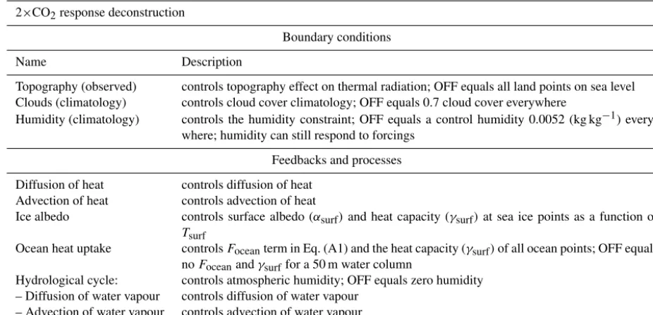
Table 1.Processes (switches) controlled in the sensitivity experiment for the mean climate deconstruction. Indentation in the left column indicates that process switches are dependent on the switches above being ON.
Mean climate deconstruction
Name Description
Ice albedo controls surface albedo (αsurf)and heat capacity (γsurf)at sea ice points as a
function ofTsurf
Clouds controls cloud cover climatology; OFF equals no clouds
Oceans controlsFoceanterm in Eq. (A1) and the heat capacity (γsurf)of all ocean points;
OFF equals noFoceanand asγsurfover land
Atmosphere: controls sensible heat flux (Fsense)and the downward atmospheric thermal
radi-ation term in Eq. (A6) – Diffusion of heat controls diffusion of heat – Advection of heat controls advection of heat – CO2 controls CO2concentration
– Hydrological cycle: controls atmospheric humidity; OFF equals zero humidity – Diffusion of water vapour controls diffusion of water vapour
– Advection of water vapour controls advection of water vapour Model corrections controls model flux correction terms
centration are switched OFF (set to zero). This marks an un-physical range of the GREB emissivity function and we will discuss the limitations of the GREB model in these experi-ments in Sect. 3b.
Diffusion of water vapour. The atmosphere transports wa-ter vapour by isotropic diffusion (third wa-term in Eq. A4). When this process is switched OFF, the term is set to zero.
Advection of water vapour. The atmosphere transports wa-ter vapour by advection following the mean wind field, u
(fifth term in Eq. A2). When this process is switched OFF, the term is set to zero.
Model corrections. The model correction terms in Eqs. (A1), (A3), and (A4) artificially force the mean Tsurf,
Tocean, andqairclimate to be as observed. When the model
correction is switched OFF, the three terms are set to zero. This will allow the GREB model to be studied without any artificial corrections and therefore help to evaluate the GREB model equations’ skill in simulating climate dynamics.
It should be noted here that the model correction terms in the GREB model have been introduced to study the response to doubling the CO2 concentration for the current climate,
which is a relatively small perturbation if compared against the other perturbations considered above. They are meaning-ful for a small perturbation in the climate system but are less likely to be meaningful with large perturbations to the cli-mate system (e.g. cloud cover set to zero).
Each different combination of the above-mentioned pro-cess switches defines a different experiment. However, not all combinations of switches are possible because some of the process switches depend on each other (see Table 1 and Fig. 1). The total number of experiments possible with these process switches is 656. For each experiment, the GREB model is run for 50 years, starting from the original GREB
model climatology, and the final year is presented as the cli-matology of this experiment in the MSCM database.
2.2 Experiments for the 2×CO2response deconstruction
In a similar way as described above for the mean climate, the climate response to a doubling of the CO2concentration
can be conceptually deconstructed with a set of GREB model experiments. These experiments help us to understand inter-actions in the climate system that lead to the climate response to a doubling of the CO2concentration. However, there are a
number of differences that need to be considered.
A meaningful deconstruction of the response to a doubling of the CO2concentration should consider the reference
trol mean climate since the forcings and the feedbacks con-trolling the response are mean state dependent. We therefore ensure that all sensitivity experiments in this discussion have the same reference mean control climate. This is achieved by estimating the flux correction term in Eqs. (A1), (A3), and (A4) for each sensitivity experiment to maintain the observed control climate. Thus, when a process is switched OFF, the control climatological tendencies in Eqs. (A1), (S3), and (S4) are the same as in the original GREB model, but changes in the tendencies due to external forcings, such as doubling the CO2concentration, are not affected by the disabled process.
This is the same approach as in DF11.
For the 2×CO2response deconstruction experiments, we
are briefly listed below (and a short summary is given in Ta-ble 2).
The following boundary conditions are considered. Topography. The topography in the GREB model affects the amount of atmosphere above the surface and therefore af-fects the emissivity of the atmosphere in the thermal radiation (Eq. A9). Regions with high topography have lower green-house gas concentrations in the thermal radiation (Eq. A9). It further affects the diffusion coefficient (κ)for the transport of heat and moisture (Eqs. A2 and A4). When the topogra-phy is turned OFF, all points of the GREB model are set to sea level height and have the same amount of CO2
concen-tration in the thermal radiation (Eq. A9).
Clouds. The cloud cover in the GREB model affects the incoming solar radiation and the emissivity of the atmo-sphere in the thermal radiation (Eq. A9). In particular, it in-fluences the sensitivity of the emissivity to changes in the CO2 concentration. A clear-sky atmosphere is more
sensi-tive to changes in the CO2concentration than a fully
cloud-covered atmosphere. When the cloud cover switch is OFF, the observed cloud cover climatology boundary conditions are replaced with a constant global mean cloud cover of 0.7. It is not set to zero to avoid an impact on the global climate sensitivity and to focus on the regional effects of inhomoge-neous cloud cover.
Humidity. Similarly to the cloud cover, the amount of at-mospheric water vapour affects the emissivity of the atmo-sphere in the thermal radiation and, in particular, the sensi-tivity to changes in the CO2concentration (Eq. A9). A
hu-mid atmosphere is less sensitive to changes in the CO2
con-centration than a dry atmosphere. When the humidity switch is OFF, the constraint to the observed humidity climatology (flux correction in Eq. A4) is replaced with a constant global mean humidity of 0.0052 kg kg−1. It is again not set to zero to avoid an impact on the global climate sensitivity and to focus on the regional effects of inhomogeneous humidity. The additional feedbacks and processes considered Ocean heat uptake. The ocean heat uptake in GREB is done in two ocean layers. The largest part of the ocean heat is in the subsurface layer,Tocean(Eq. A3). When the ocean switch
is OFF theFocean term in Eq. (A1) is set to zero, Eq. (A3) is
set to zero, and the heat capacity (γsurf)of all ocean points in
Eq. (A1) is set to that of a 50 m water column.
The total number of experiments with these process switches is 640. For each experiment, the GREB model is run for 50 years, starting from the original GREB model clima-tology, with a doubling of the CO2concentrations in the first
time step. The changes over the 50-year period relative to the original GREB model climatology of these experiments are presented in the MSCM database.
2.3 Scenario experiments
There are a number of different scenarios for external bound-ary condition changes in the MSCM experiment database. They include different changes in the CO2concentration and
in the incoming solar radiation. A complete overview is given in Table 3. A short description follows below.
2.3.1 RCP scenarios
In the Representative Concentration Pathway (RCP) scenar-ios the GREB model is forced with time-varying CO2
con-centrations. All five different simulations have the same his-torical time evolution of CO2 concentrations starting from
1850 to 2000, and from 2001 the follow the RCP8.5, RCP6, RCP4.5, RCP2.6, and A1B CO2concentration pathways
un-til 2100 (van Vuuren et al., 2011). 2.3.2 Idealized CO2scenarios
The 15 idealized CO2concentration scenarios in the MSCM
experiment database focus on the non-linear time delay and regional differences in the climate response to different CO2concentrations. These were implemented in five
simula-tions in which the control CO2concentration (340 ppm) was
changed in the first time step to a scaled CO2concentration
of 0, 0.5, 2, 4, and 10 times the control level. The 0.5×CO2
and 2×CO2simulations are 50 years long and the others are
100 years long.
Two different simulations with idealized time evolutions of CO2 concentrations are conducted to study the time
de-lay of the climate response. In one simulation, the CO2
con-centration is doubled in the first time step, held at this level for 30 years, and then returned to control levels instanta-neously (2×CO2 abrupt reverse). In the second simulation,
the CO2 concentration is varied between the control and
2×CO2concentrations following a sine function with a
pe-riod of 30 years, starting at the minimum of the sine function at the control CO2concentration (2×CO2wave). Both
sim-ulations are 100 years long.
The third set of idealized CO2 concentration scenarios
double the CO2concentrations restricted to different regions
or seasons. The eight regions and seasons include the North-ern or SouthNorth-ern Hemisphere, the tropics (30◦S–30◦N) or ex-tratropics (poleward of 30◦), land or oceans, and the months October to March or April to September. Each experiment is 50 years long.
2.3.3 Solar radiation
Two different experiments with changes in the solar constant were created. In the first experiment, the solar constant is increased by about 2 % (+27 W m−2), which leads to about the same global warming as a doubling of the CO2
pe-Table 2.Processes (switches) controlled in the sensitivity experiment for the 2×CO2response deconstruction. Indentation in the left column indicates that process switches are dependent on the switches above being ON.
2×CO2response deconstruction
Boundary conditions Name Description
Topography (observed) controls topography effect on thermal radiation; OFF equals all land points on sea level Clouds (climatology) controls cloud cover climatology; OFF equals 0.7 cloud cover everywhere
Humidity (climatology) controls the humidity constraint; OFF equals a control humidity 0.0052 (kg kg−1) every-where; humidity can still respond to forcings
Feedbacks and processes Diffusion of heat controls diffusion of heat
Advection of heat controls advection of heat
Ice albedo controls surface albedo (αsurf)and heat capacity (γsurf)at sea ice points as a function of
Tsurf
Ocean heat uptake controlsFoceanterm in Eq. (A1) and the heat capacity (γsurf)of all ocean points; OFF equals
noFoceanandγsurffor a 50 m water column
Hydrological cycle: controls atmospheric humidity; OFF equals zero humidity – Diffusion of water vapour controls diffusion of water vapour
– Advection of water vapour controls advection of water vapour
riod of 11 years, representing an idealized variation of the in-coming solar short-wave radiation due to the natural 11-year solar cycle (Willson and Hudson, 1991). Both experiments are 50 years long.
2.3.4 Idealized orbital parameters
A series of five simulations are done in the context of orbital forcings and the related ice age cycles. In one simulation, the incoming solar radiation as a function of latitude and day of the year was changed to its values from 231 kyr ago (Berger and Loutre, 1991; Huybers, 2006). In an additional simula-tion, the CO2concentration is reduced from 340 to 200 ppm
as observed during the peak of ice age phases in combination with the incoming solar radiation changes. Both simulations are 100 years long.
In three sensitivity experiments, we changed the incom-ing solar radiation accordincom-ing to some idealized orbital pa-rameter changes to study the effect of the most important orbital parameters. The orbital parameters changed are the distance to the Sun, the Earth axis tilt relative to the Earth– Sun plane (obliquity), and the eccentricity of the Earth orbit around the Sun. The orbit radius was changed from 0.8 to 1.2 AU in steps of 0.01 AU, the obliquity from −25 to 90◦ in steps of 2.5◦, and the eccentricity from 0.3 (Earth clos-est to the Sun in July) to 0.3 (Earth furthclos-est from the Sun in July) in steps of 0.01. Each sensitivity experiment was started from the control GREB model (1AU radius, 23.5◦obliquity, and 0.017 eccentricity) and run for 50 years. The last year of each simulation is presented as the estimate for the equilib-rium climate.
3 Some results of the model simulations
The MSCM experiment database includes a large set of ex-periments that address many different aspects of the climate. At the same time, the GREB model has limited complexity and not all aspects of the climate system are simulated in the GREB experiments. The following analysis will give a short overview of some of the results that can be taken from the MSCM experiments. In this we will focus on aspects of general interest and on comparing the outcome to results of other published studies to illustrate the strengths and limi-tations of the GREB model in this context. The discussion, however, will be incomplete, as there are simply too many aspects that could be discussed in this set of experiments. We will therefore focus on a general introduction and leave space for future studies to address other aspects.
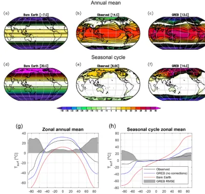
3.1 GREB model performance
The skill of the GREB model is illustrated in Fig. 4 by run-ning the GREB model without the correction terms. For ref-erence, we compare this GREB run with the observed mean climate and seasonal cycle (this is identical to running the GREB model with correction terms) and with a bare world. The latter is the GREB model with all switches OFF (radia-tive balance without an atmosphere and a dark surface). In comparison with the full GREB model, this illustrates how much all the climate processes affect the climate.
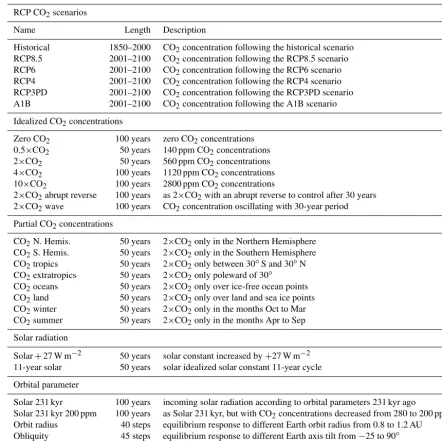
struc-Table 3.List of scenario experiments.
RCP CO2scenarios
Name Length Description
Historical 1850–2000 CO2concentration following the historical scenario
RCP8.5 2001–2100 CO2concentration following the RCP8.5 scenario
RCP6 2001–2100 CO2concentration following the RCP6 scenario
RCP4 2001–2100 CO2concentration following the RCP4 scenario
RCP3PD 2001–2100 CO2concentration following the RCP3PD scenario
A1B 2001–2100 CO2concentration following the A1B scenario Idealized CO2concentrations
Zero CO2 100 years zero CO2concentrations 0.5×CO2 50 years 140 ppm CO2concentrations
2×CO2 50 years 560 ppm CO2concentrations 4×CO2 100 years 1120 ppm CO2concentrations
10×CO2 100 years 2800 ppm CO2concentrations
2×CO2abrupt reverse 100 years as 2×CO2with an abrupt reverse to control after 30 years
2×CO2wave 100 years CO2concentration oscillating with 30-year period
Partial CO2concentrations
CO2N. Hemis. 50 years 2×CO2only in the Northern Hemisphere
CO2S. Hemis. 50 years 2×CO2only in the Southern Hemisphere
CO2tropics 50 years 2×CO2only between 30◦S and 30◦N
CO2extratropics 50 years 2×CO2only poleward of 30◦
CO2oceans 50 years 2×CO2only over ice-free ocean points
CO2land 50 years 2×CO2only over land and sea ice points CO2winter 50 years 2×CO2only in the months Oct to Mar
CO2summer 50 years 2×CO2only in the months Apr to Sep
Solar radiation
Solar+27 W m−2 50 years solar constant increased by+27 W m−2 11-year solar 50 years solar idealized solar constant 11-year cycle Orbital parameter
Solar 231 kyr 100 years incoming solar radiation according to orbital parameters 231 kyr ago
Solar 231 kyr 200 ppm 100 years as Solar 231 kyr, but with CO2concentrations decreased from 280 to 200 ppm Orbit radius 40 steps equilibrium response to different Earth orbit radius from 0.8 to 1.2 AU Obliquity 45 steps equilibrium response to different Earth axis tilt from−25 to 90◦ Eccentricity 60 steps equilibrium response to different Earth orbit eccentricity from 0.3 to 0.3
ture within Asia or zonal temperature gradients within ocean basins). For most of the globe (<50◦from the Equator), the GREB model root mean square error (RMSE) for the annual mean Tsurf is less than 10◦C relative to the observed (see
Fig. 4g). This is larger than for state-of-the-art CMIP-type climate models, which typically have an RMSE of about 2◦C (Dommenget, 2012). In particular, the regions near the poles have high RMSE. It seems likely that the meridional heat transport is the main limitation in the GREB model given tropical regions that are too warm, polar regions that are gen-erally too cold, and a seasonal cycle in the polar regions that is too strong in the GREB model without correction terms.
The GREB model performance can be put in perspective by illustrating how much the climate processes simulated in
the GREB model contribute to the mean climate relative to the bare world simulation (see Fig. 4). The GREB RMSE to observed is about 20 %–30 % of the RMSE of the bare world simulation (not shown), suggesting that the GREB model has a relative error of about 20 %–30 % in the pro-cesses that it simulates or due to propro-cesses that it does not simulate (e.g. ocean heat transport).
3.2 Mean climate deconstruction
esti-Figure 4.Tsurfannual mean(a, b, c)and seasonal cycle (half the difference between mean of July to September minus January to March;d, c, f) for the GREB experiment with all processes turned OFF (bare Earth), only the correction term OFF (GREB), and observed (identical to GREB with all processes ON). The zonal mean of the annual mean(g)and seasonal cycle(h)of the experiments and observations in comparison with the zonal mean RMSE of the GREB model without correction terms relative to observed.
mate for climate sensitivity (Knutti et al., 2006). In the fol-lowing analysis, we will give a short overview of how the 10 processes of the MSCM experiments contribute to the mean climate and its seasonal cycle. For these experiments, we use the GREB model without flux correction terms.
In the discussion of the experiments, it is important to con-sider the fact that climate feedbacks are contributing to the interactions of climate processes. The effect of a climate pro-cess on the climate is a result of all the other active climate processes responding to the changes that the climate pro-cess under consideration introduces. It also depends on the mean background climate. Therefore, the particular combi-nation of switches with which GREB model experiments are discussed does matter. For instance, the effect of ice–snow cover is stronger in a much colder background climate, but it is also affected by feedback in other climate processes, such
as the water vapour feedback. We will therefore consider dif-ferent experiments or difdif-ferent experiment sets to shed some light on these interactions.
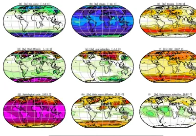
In Figs. 5 and 6 the contributions of each of the 10 pro-cesses (except the atmosphere) to the annual mean climate (Fig. 5) and its seasonal cycle (Fig. 6) are shown. In each ex-periment, all processes are active, but the process of interest and the model correction terms are turned OFF. The results are compared against the complete GREB model without the model correction terms (all processes active; expect model correction terms). For the hydrological cycle we will discuss some additional experiments in which the ice–albedo feed-back is turned OFF as well.
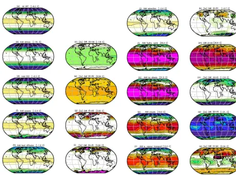
Figure 5.Changes in the annual meanTsurfin the GREB model simulations with different processes turned OFF as described in Sect. 2a
relative to the complete GREB model without model correction terms:(a)ice–snow,(b)clouds,(c)oceans,(d)heat advection,(e)heat diffusion,(f)CO2concentration,(g)hydrological cycle,(h)diffusion of water vapour, and(i)advection of water vapour. Global mean
differ-ences are shown in the headings. Differdiffer-ences are for the control minus the sensitivity experiment (positive indicates the control experiment is warmer). All values are in degrees Celsius (◦C). In some panels, the values are scaled for better comparison:(b),(c), and(f)by a factor of 2;(a),(d), and(e)by a factor of 3; and(h)and(i)by a factor of 6.
shown) the insulation effect of the sea ice actually leads to warming, as the ocean cannot cool down as much during win-ter as it does without sea ice.
The cloud cover in the GREB model is only considered as a given boundary condition but does not simulate the for-mation of clouds. Therefore, it does not include cloud feed-backs. However, mean cloud cover influences the radiation balance of solar and thermal radiation and therefore affects the mean climate and its seasonal cycle. Figure 5b illustrates the fact that cloud cover has a large net cooling effect glob-ally due to the solar radiation reflection effect dominating over the thermal radiation warming effect. Previous studies on the cloud cover effect on the overall climate mostly focus on radiative forcings estimates, but to our best knowledge, they do not discuss how much the mean surface tempera-ture is affected by the mean cloud cover (e.g. Rossow and Zhang, 1995).
It is interesting to note that the strongest cooling effect of cloud cover is over regions with fairly little cloud cover (e.g. deserts and mountain regions). Here it is important to point out that the climate system response to any external forcing or changes in the boundary conditions, such as CO2
forcing or removing the cloud cover, is dominated by
inter-nal positive feedback rather than the direct local forcing ef-fect (e.g. see the discussion of the global warming pattern in DF11).
The most important internal positive feedback is the water vapour feedback, which amplifies the effect of removing the cloud cover. This feedback is stronger over dry and cold re-gions (DF11) and therefore amplifies the effects of removing the cloud cover over deserts and mountain regions.
The large ocean heat capacity slows down the seasonal cycle (Fig. 6c). Subsequently, the seasons are more moder-ate than they would be without the ocean transferring heat from warm to cold seasons. This is, in particular, important in the middle and higher latitudes. The effect of the ocean heat capacity, however, also has an annual mean warming effect (Fig. 5c). This is due to the non-linear thermal radiation cool-ing. The non-linear black-body negative radiation feedback is stronger for warmer temperatures, which are not reached in a moderated seasonal cycle with the larger ocean heat capac-ity. Studies with more complex climate models find similar impacts of the ocean heat capacity on the annual mean and seasonal cycle (e.g. Donohoe et al., 2014).
po-Figure 6.As in Fig. 5, but for the seasonal cycle. The mean seasonal cycle is defined by the difference between the months (JAS – JFM) divided by two. Positive values on the Northern Hemisphere indicate a stronger seasonal cycle in the sensitivity experiments than in the full GREB model and vice versa for the Southern Hemisphere. Global root mean square differences are shown in the headings. All values are in degrees Celsius (◦C). In some panels, the values are scaled for better comparison:(b),(d), and(e)by a factor of 2; and(h)and(i)by a factor of 10.(g)The mean for the hydrological cycle experiments with and without the ice–albedo process active.
lar regions) and cools the hottest regions (e.g. warm deserts). In global averages, this is mostly cancelled out. The advec-tion of heat has strong effects where the mean winds blow across strong temperature gradients. This is mostly present in the Northern Hemisphere (Fig. 5e). The most prominent feature is the strong warming of the northern European and Asian continents in the cold season. On global average, warming and cooling mostly cancel each other out.
Literature discussions of heat transport are usually based on heat budget analysis of the climate system (in obser-vations or simulations) instead of “switching off” the heat transport in fully complex climate models, since such exper-iments are difficult to conduct. A similar heat budget analy-sis of the GREB model experiments is beyond the scope of this study, but the results of these experiments appear to be largely consistent with the findings of heat budget analyses. For instance, the regional contributions of diffusion and ad-vection are similar to those found in previous studies (e.g. Peixoto and Oort, 1992; Yang et al., 2015).
The CO2concentration leads to a global mean warming of
about 9◦C (Fig. 5f). Even though it is the same CO2
concen-tration everywhere, the warming effect is different at differ-ent locations. This is discussed in more detail in DF11 and in Sect. 3c.
The input of water vapour into the atmosphere by the hy-drological cycle leads to a substantial amount of warming globally (Fig. 5g). However, we need to consider the fact that the experiment with switching OFF the hydrological cycle is the only experiment in which we have a significant amount of global cooling (by about−44◦C). As a result, most of the Earth is below freezing temperatures and therefore has a much stronger ice–albedo feedback than in any other ex-periment. This leads to a significant amplification of the re-sponse.
Similar to the oceans, the hydrological cycle dampens the seasonal cycle (Fig. 6g), but with a much weaker ampli-tude. The transport of water vapour away from warm and moist regions (e.g. tropical oceans) to cold and dry regions (e.g. high latitudes and continents) leads to additional warm-ing in the regions that gain water vapour and coolwarm-ing in those that lose water vapour (Fig. 6h). The effect is similar in both hemispheres. The transport of water vapour along the mean wind directions has stronger effects on the Northern Hemi-sphere than on the Southern HemiHemi-sphere, since the northern hemispheric mean winds have more of a meridional compo-nent, which creates advection across water vapour gradients (Fig. 6i). This effect is most pronounced in the cold seasons. Most processes have a predominately zonal structure. We can therefore take a closer look at the zonal mean climate and seasonal cycle of all processes to get a good represen-tation of the relative importance of each process; see Fig. 7. The annual mean climate is most strongly influenced by the hydrological cycle (here shown as the mean of the response with and without the ice–albedo feedback). The cloud cover has an opposing cooling effect but is weaker than the warm-ing effect of the hydrological cycle. The warmwarm-ing effect by the ocean’s heat capacity is similar in scale to that of the CO2
concentration.
An interesting aspect of the climate system is that the Northern Hemisphere is warmer than the southern counter-part (by about 1.5◦C; not shown), which may be counterin-tuitive given the warming effect of the ocean heat capacity (see above discussion; Kang et al., 2015). The GREB model without flux correction also has a warmer Northern Hemi-sphere than the southern counterpart (by about 0.3◦C; not shown), whereas the bare Earth (pure black-body radiation balance; GREB all switches OFF) would have the Northern Hemisphere colder than the southern counterpart (by about −0.6◦C; not shown). A number of processes play into this inter-hemispheric contrast, with the most important contri-bution coming from cross-equatorial heat and moisture ad-vection (see Fig. 7a). This is largely consistent with Kang et al. (2015).
The seasonal cycle is damped most strongly by the ocean’s heat capacity and by the hydrological cycle. The latter may seem unexpected but is due to the effect of increased water vapour having a stronger warming effect in the cold seasons, similarly to the greenhouse effect of CO2concentrations. In
turn, ice–snow cover and cloud cover lead to an intensifica-tion of the seasonal cycle at higher latitudes. Again, the latter may seem unexpected but is due to interaction with other cli-mate feedbacks such as the water vapour feedback, which also makes the climate more strongly respond to changes in cloud cover in regions where there actually is very little cloud cover (e.g. deserts).
As an alternative way of understanding the role of the dif-ferent process we can build up the complete climate by intro-ducing one process after the other; see Figs. 8 and 9. We start with the bare Earth (e.g. like our Moon) and then introduce
one process after the other. The order in which the processes are introduced is mostly motivated by giving a good repre-sentation of each of the 10 processes. However, it can also be interpreted as a build-up of the Earth climate in a somewhat historical way: we assume that initially the Earth was a bare planet and then the atmosphere, ocean, and all other aspects were built up over time.
The bare Earth (all switches OFF) is a planet without at-mosphere, ocean, or ice. It has an extremely strong seasonal cycle (Fig. 9a) and is much colder than our current climate (Fig. 8a). It also has no regional structure other than merid-ional temperature gradients. The combination of all climate processes will create most of the regional and seasonal dif-ferences that make up our current climate.
The atmospheric layer in the GREB model simulates two processes if all other processes are turned off: a turbulent sensible heat exchange with the surface and thermal radia-tion due to residual trace gases other than CO2, water vapour,
or clouds. However, as mentioned in Appendix A1 the log-function approximation leads to negative emissivity if all greenhouse gas (CO2and water vapour) concentrations and
cloud cover are zero. The negative emissivity turns the atmo-spheric layer into a cooling effect, which dominates the im-pact of the atmosphere in this experiment (Fig. 8b, c). This is a limitation of the GREB model and the result of this ex-periment as such should be considered with caution. In a more realistic experiment we can set the emissivity of the atmosphere to zero or a very small value (0.01) to simulate the effect of the atmosphere without CO2, water vapour, and
cloud cover; see Fig. S2. Both experiments have very simi-lar warming effects in posimi-lar regions, suggesting that sensible heat exchange warms the surface. The residual thermal ra-diation effect from the emissivity of 0.01 has only a minor impact (Fig. S2f and g).
The warming effect of the CO2 concentration is nearly
uniform (Fig. 8d, e) and without much of a seasonal cycle (Fig. 9d, e) if all other processes are turned OFF. This ac-counts for a warming of about+9◦C.
The large ocean heat capacity reduces the amplitude of the seasonal cycle (Fig. 9f, g). The effective heat capacity of the oceans is proportional to the observed mixed layer in the GREB model, which causes some small variations (dif-ferences from the zonal means) as seen in the seasonal cy-cle of the oceans. Land points are not affected, since there is no atmospheric transport (advection and diffusion turned OFF). The different heat capacity between oceans and land is already a significant element of the regional and seasonal climate differences (Fig. 8f, g).
Figure 7.Zonal mean values of the annual mean(a)and seasonal cycle differences(b)for the experiments as shown in Figs. 5 and 6g. The mean for the hydrological cycle is for the experiments with and without the ice–albedo process active.
Figure 8.Conceptual build-up of the annual mean climate starting with all processes turned OFF(a)and then adding more processes in each row:(b)atmosphere,(d)CO2,(f)oceans,(h)heat diffusion,(j)heat advection,(l)hydrological cycle,(n)ice albedo,(p)clouds, and
Figure 9.As in Fig. 8, but conceptual build-up of the seasonal cycle. The seasonal cycle is defined by the difference between the months (JAS – JFM) divided by two. Global mean absolute values are shown in the heading. In some panels the values are scaled for better comparison:
(c),(i),(m), and(o)by a factor of 2;(k),(q), and(s)by a factor of 5; and(e)by a factor of 30.
with lower latitudes. The turbulent heat exchange makes re-gional climate differences a bit more realistic.
The advection of heat is strongly dependent on the tem-perature gradients along the mean wind field directions. It provides substantial heating during the winter season for Eu-rope, Russia, and western North America (Figs. 8j, k, 9j, k). The structure (differences from the zonal mean) created by this process is mostly caused by the prescribed mean wind climatology. In particular, the milder climate in Europe com-pared to northeast Asia at the same latitudes is created by wind blowing from the ocean onto land. The same is true for the differences between the west and east coasts of northern North America. The climate regional and seasonal structures are now quite realistic, but the overall climate is much too cold. The ice–snow cover further cools the climate, in partic-ular the polar regions (Fig. 8n, o). This difference illustrates the fact that the ice–albedo feedback primarily leads to cool-ing in higher latitudes and mostly in the winter season.
Introducing the hydrological cycle brings the most impor-tant greenhouse gas into the atmosphere: water vapour. This
has an enormous warming effect globally (Fig. 8l, m) with a moderate reduction in the strength of the seasonal cycle (Fig. 9l, m). The resulting modelled climate is now much too warm, but introducing cloud cover cools the climate substan-tially (Fig. 8p, q) and leads to a fairly realistic climate.
The atmospheric transport (diffusion and advection) brings water vapour from relatively moist regions to rela-tively dry regions (Fig. 8r, s). This leads to enhanced warm-ing in the dry and cold regions (e.g. the Sahara or polar re-gions) by the water vapour thermal radiation (greenhouse) effect and cooling in the regions where it came from (e.g. tropical oceans). The heating effect is similar to the transport of heat and also has a strong seasonal cycle component.
heat capacity, but the resulting changes in surface temper-ature gradients will also affect the atmospheric circulation patterns and subsequently the cloud cover. Such effects on the atmospheric circulation and cloud cover are neglected in the GREB model, as they are given as fixed boundary condi-tions. Regionally, such effects can be significant and CGCM simulations are required to study such effects.
3.3 2×CO2response deconstruction
The doubling of the CO2 concentrations leads to a distinct
warming pattern with polar amplification, a land–sea con-trast, and significant seasonal differences in the warming rate. These structures in the warming pattern reflect complex interactions between feedbacks in the climate system and re-gional differences in the CO2 forcing pattern. The MSCM
2×CO2response experiments are designed to help us
under-stand the interactions causing this distinct warming pattern. DF11 discussed many aspects of these experiments with a focus on the land–sea contrast, the seasonal differences, and the polar amplification. We will therefore focus here only on some aspects that have not been previously discussed in DF11.
In the GREB model, we can turn OFF the atmospheric transport and thereby study the local interaction without any lateral interactions. Figure 10 shows three experiments in which the atmospheric transport and other processes (see fig-ure caption) are inactive. The three experiments highlight the regional difference in the CO2forcing pattern and in the two
main feedbacks (water vapour and ice albedo).
In the first experiment (Fig. 10a) without feedback pro-cesses, the localTsurfresponse is approximately directly
pro-portional to the local CO2forcing. The regional differences
are caused by differences in cloud cover and atmospheric hu-midity, since both influence the thermal radiation effect of CO2(DF11; Kiehl and Ramanathan, 1982; Cess et al., 1993).
This causes, on average, the land regions to see a stronger forcing than oceanic regions (see Fig. 10b). However, even over oceans we can see clear differences. For instance, the warm pool of the western tropical Pacific sees less CO2
forc-ing than the eastern tropical Pacific.
The ice–albedo feedback is strongly localized, and it is strongest over the mid-latitudes of the northern continents and at the sea ice edge around Antarctica (Fig. 10c and d). The water vapour feedback is far more widespread and stronger (Fig. 10e and f). It is strongest in relatively warm and dry regions (e.g. subtropical oceans) but also shows some clear localized features, such as strong Arabian and Mediter-ranean Sea warming.
3.4 Scenarios
The set of scenario experiments in the MSCM simulations allows us to study the response of the climate system to changes in the external boundary conditions in a number of
Figure 10.LocalTsurfresponse to doubling of the CO2 concentra-tion in experiments without atmospheric transport (each point on the maps is independent of the others).(a)GREB with topography, humidity, cloud processes, and all other processes OFF.(b) Differ-ence of(a)to GREB with topography and all other processes OFF scaled by a factor of 10.(c)GREB model as in(a), but with the ice–albedo process ON.(d)Difference of(c–a)scaled by a factor of 2.(e)GREB model as in(a), but with hydrological cycle process ON.(f)Difference of(e–a)scaled by a factor of 2. For details on the experiments, see Sect. 2b.
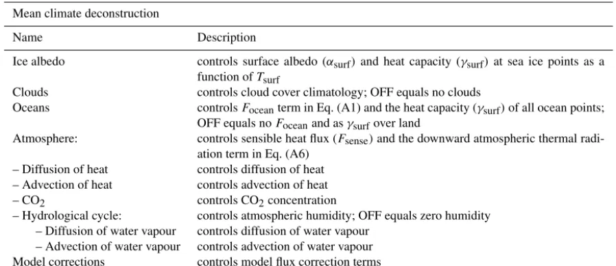
different ways. In the following, we will briefly illustrate some results from these scenarios and organize the discus-sion by the different themes in scenario experiments.
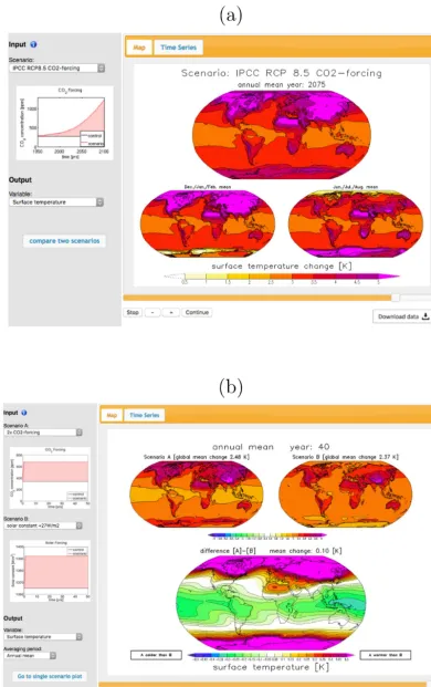
The CMIP has defined a number of standard CO2
concen-tration projection simulations that give different RCP scenar-ios for future climate change; see Fig. 11a. The GREB model sensitivity in these scenarios is similar to those of the CMIP database (Forster et al., 2013).
Idealized CO2concentration scenarios help us to
under-stand the response to the CO2forcing. In Fig. 11b, we show
the global meanTsurfresponse to different scaling factors of
CO2concentrations. To first order, we can see that the global
meanTsurfresponse follows a logarithmic CO2concentration
(e.g. any doubling of the CO2concentration leads to the same
global meanTsurf response; compare 2×CO2 with 4×CO2
or with Fig. 11b) as suggested in other studies (Myhre et al., 1998). However, this relationship does break down if we go to very low CO2 concentrations (e.g. zero CO2
concentra-tion), illustrating the fact that the log-function approximation of the CO2forcing effect is only valid within a narrow range
Figure 11.Global meanTsurfresponse to idealized forcing
scenar-ios:(a)different RCP CO2forcing scenarios.(b)Scaled CO2
con-centrations.(c)Idealized CO2concentration time evolutions (dot-ted lines) and the respectiveTsurfresponses (solid lines of the same
colour) for the 2×CO2abrupt reverse (red) and the 2×CO2wave
(blue) simulations.(d)Idealized 11-year solar cycle. The list of ex-periments is given in Table 3.
The transient response time to CO2 forcing can be
es-timated from idealized CO2 concentration changes; see
Fig. 11c. The stepwise change in CO2 concentration
illus-trates the response time of the global climate. In the GREB model, it takes about 10 years to get 80 % of the response to a CO2concentration change (see step function response;
Fig. 11c). In turn, the response to a CO2concentration wave
time evolution is a lag of about 3 years. The fast versus slow response also leads to different warming patterns with strong land–sea contrasts (not shown) that are largely similar to those found in previous studies (Held et al., 2010).
The regional aspects of the response to a CO2
concen-tration can also be studied by partially increasing the CO2
concentration in different regions; see Fig. 12. The warm-ing response mostly follows the regions where we partially changed the CO2concentration, but there are some
interest-ing variations in this. The partial increase in the CO2
concen-tration over oceans has a stronger warming impact than the partial increase in the CO2concentration over land for most
Southern Hemisphere land regions. In turn, the land forcing has little impact for the ocean regions. The boreal winter forcing has a stronger impact on the Southern Hemisphere than boreal summer forcing, suggesting that the warm son forcing is, in general, more important than the cold sea-son forcing. The only exception to this is the Tibetan Plateau region.
A series of scenarios focus on the impact of solar forc-ing. In Fig. 11d, we show the response to an idealized 11-year solar cycle. The global mean Tsurf response is 2
or-ders of magnitude smaller than the response to a doubling of the CO2concentration, reflecting the weak amplitude of this
forcing. This result is largely consistent with the response found in GCM simulations (Cubasch et al., 1997) but does not consider possible more complicated amplification mech-anisms (Meehl et al., 2009). A change in the solar constant of+27 W m−2 has a globalTsurf warming response similar
to a doubling of the CO2concentration but with a slightly
different warming pattern; see Fig. 13. The warming pat-tern of a solar constant change has a stronger warming when incoming sunlight is stronger (e.g. tropics or summer sea-son) and a weaker warming in regions with less incoming sunlight (e.g. higher latitudes or winter season). This is in general agreement with other modelling studies (Hansen et al., 1997).
On longer paleo-timescales (>10 000 years), changes in the orbital parameters affect the incoming sunlight. Figure 14 illustrates the response to a number of orbital solar radia-tion changes. Incoming radiaradia-tion (sunlight) typical of the ice age (231 kyr ago) has less incoming sunlight in the north-ern hemispheric summer. However, it has every little annual global mean change (Fig. 14a) due to increases in sunlight over other regions and seasons. TheTsurf response pattern
in the zonal mean in different seasons is very similar to the solar forcing, but the response is slightly more zonal and sea-sonal differences are less dominant (Fig. 14b). The response is also amplified at higher latitudes. However, in the global mean there is no significant global cooling as observed dur-ing ice ages. If the solar forcdur-ing is combined with a reduction in the CO2 concentration (from 340 to 200 ppm), we find
a global mean cooling of−1.7◦C (Fig. 14c), which is still much weaker than observed during ice ages but is largely consistent with previous simulations of ice age conditions (Weaver et al., 1998; Braconnot et al., 2007). This is not un-expected since the GREB model does not include an ice sheet model and, therefore, does not include glacier growth feed-backs that would amplify ice age cycles.
A better understanding of the orbital solar radiation forc-ing can be gained by analysforc-ing the response to idealized or-bital parameter changes. We therefore vary the Earth distance to the Sun (radius), the Earth axis tilt to the Earth orbit plane (obliquity), and the shape of the Earth orbit around the Sun (eccentricity) over a wider range; see Fig. 14d–f. When the radius is changed by 10 %, the Earth climate becomes es-sentially uninhabitable, with either global mean temperature above 30◦C (approx. summer mean temperature of the Sa-hara) or a completely ice-covered snowball Earth. This sug-gests that the habitable zone of the Earth radius is fairly small due to the positive feedbacks within the climate system simu-lated in the GREB model (not considering long-term or more complex atmospheric chemistry feedbacks) and largely con-sistent with previous studies (Kasting et al., 1993).
Figure 12.Tsurfresponse to partial doubling of the CO2concentration in the Northern(a)and Southern(b)Hemisphere, the tropics(d),
extratropics(e), oceans(g), land(h), boreal winter(j), and summer(k). The right column shows the difference between the two panels to the left in the same row.
year. In the extreme case, when the obliquity is 90◦, the trop-ics become ice covered and cooler than the polar regions, which are now warmer than the tropics today and ice free. The polar regions now have an extreme seasonal cycle (not shown), with sunlight all day during summer and no sunlight during winter. Any eccentricity increase in amplitude would lead to a warmer overall climate. Thus, a perfect-circle orbit around the Sun has, on average, the coldest climate, and all of the more extreme eccentricity (elliptic) orbits have warmer climates. This suggests that the warming effect of the sec-tion of the orbit that has a closer transit around the Sun in an eccentricity orbit relative to the perfect-circle orbit over-compensates for the cooling effect of the more remote transit around the Sun in the other half of the orbit relative to the perfect-circle orbit.
4 Summary and discussion
In this study, we introduced the MSCM database (version: MSCM-DB v1.0) for research analysis with more than 1300 experiments. It is based on simulations with the GREB model for studies of the processes that contribute to the mean cli-mate, the response to doubling the CO2concentration, and
different scenarios with CO2or solar radiation forcings. The
GREB model is a simple climate model that does not sim-ulate internal weather variability, circulation, or cloud cover changes (feedbacks). It provides a simple and fast null hy-pothesis for interactions in the climate system and its re-sponse to external forcings.
pro-Figure 13.Tsurfresponse to changes in the solar constant by+27 W m−2(b, e)versus a doubling of the CO2concentration(a, d)for the
annual mean(a, c, c)and the seasonal cycle(d, e, f). The seasonal cycle is defined by the difference between the months (JAS – JFM) divided by two.(c, f)The difference between panels(a)and(b)and between panels(d)and(e), respectively, scaled by 4(c)and 3(f).
cesses the RMSE is reduced to about 20 %–30 % relative to observed. Further, the GREB model emissivity function reaches unphysical negative values when water vapour, CO2,
and cloud cover are set to zero. This is a limitation of the log-function parameterization that can potentially be revised if a new parameterization is developed that considers these cases. However, it is beyond the scope of this study to develop such a new parameterization and it is left for future studies.
The MSCM experiments for the conceptual deconstruction of the observed mean climate provide a good understanding of the processes that control the annual mean climate and its seasonal cycle. The cloud cover, atmospheric water vapour, and ocean heat capacity are the most important processes that determine the regional difference in the annual mean cli-mate and its seasonal cycle. The observed seasonal cycle is strongly damped not only by the ocean heat capacity, but also by the water vapour feedback. In turn, ice albedo and cloud cover amplify the seasonal cycle in higher latitudes.
The conceptual deconstruction of the response to a dou-bling of the CO2concentration based on the MSCM
exper-iments has mostly been discussed in DF11, but some addi-tional results shown here focus on the local forcing in re-sponses without horizontal interaction. It has been shown here that the CO2forcing has a clear land–sea contrast,
sup-porting the land–sea contrast in theTsurfresponse. The water
vapour feedback is widespread and most dominant over the subtropical oceans, whereas the ice–albedo feedback is more localized over northern hemispheric continents and around the sea ice border.
The series of scenario simulations with CO2 and solar
forcing provide many useful experiments to understand dif-ferent aspects of the climate response. The RCP and ideal-ized CO2forcing scenarios give good insights into climate
sensitivity, regional differences, transient effects, and the role of CO2forcing in different seasons or at different locations.
The solar forcing experiments illustrate the subtle differences in the warming pattern of CO2forcing, and the orbital solar
forcing experiments illustrated elements of the climate re-sponse to long-term paleoclimate forcings.
Figure 14.Orbital parameter forcings andTsurfresponses:(a)incoming solar radiation changes in the solar 231 kyr experiment relative to
the control GREB model.Tsurfresponse in solar 231 kyr(b)and solar 231 kyr 200 ppm(c)relative to the control GREB model. Annual mean
Tsurfin orbit radius(d), obliquity(e), and eccentricity(f). The solid vertical line in(d–f)marks the control (today) GREB model.
or socio-economic impacts require more complex climate models.
Future development of this MSCM database will continue and it is expected that this database will grow. The devel-opment will go in several directions: the GREB model per-formance in the processes that it currently simulates will be further improved. In particular, the simulation of the hydro-logical cycle needs to be improved to allow for the use of the GREB model to study changes in precipitation. Simu-lations of aspects of the large-scale atmospheric circulation, aerosols, carbon cycle, and glaciers would further enhance the GREB model and would provide a wider range of exper-iments to run for the MSCM database.
Code and data availability. The MSCM model code, including all required input files, to do all the experiments described on the MSCM home page and in this paper can be down-loaded as a compressed tar archive from the MSCM home page under http://mscm.dkrz.de/download/mscm-web-code.tar.gz (last access: 3 November 2018) or from the bitbucket repos-itory under https://bitbucket.org/tobiasbayr/mscm-web-code (last access: 3 November 2018). The data for all the experiments of the MSCM can be accessed via the MSCM web page interface (DOI: https://doi.org/10.4225/03/5a8cadac8db60; Dom-menget, 2018). The mean deconstruction experiment file names have an 11-digit binary code that describes the 11 process switch
combinations: 1: ON and 0: OFF. The digits from left to right present the following processes.
1. Model corrections 2. Ice albedo 3. Cloud cover
4. Advection of water vapour 5. Diffusion of water vapour 6. Hydrologic cycle 7. Ocean
8. CO2
9. Advection of heat 10. Diffusion of heat 11. Atmosphere
For example, the data filegreb.mean.decon.exp-10111111111.gad
is the experiment with all processes ON, but ice albedo is OFF. The 2×CO2response deconstruction experiment file names have a
10-digit binary code that describes the 10 process switch combinations. The digits from left to right present the following processes.
6. Advection of heat 7. Diffusion of heat 8. Humidity (climatology) 9. Clouds (climatology) 10. Topography (observed)
For example, the data fileresponse.exp-0111111111.2xCO2.gadis the experiment with all processes ON, but ocean heat uptake is OFF. The individual experiments can be chosen from the web page inter-face by selecting the desired switch combinations. Alternatively, all experiments can be downloaded in a combined tar file from the web page interface.
Appendix A: GREB model equations
Table A1.Variables of the GREB model equations.
Variable Dimensions Description
Tsurf x,y,t surface temperature
Tatmos x,y,t atmospheric temperature
Tocean x,y,t subsurface ocean temperature
qair x,y,t atmospheric humidity
γsurf x,y,t heat capacity of the surface layer
γatmos x,y,t heat capacity of the atmosphere
γocean x,y,t heat capacity of the subsurface ocean
Fsolar x,y,t solar radiation absorbed at the surface
Fthermal x,y,t thermal radiation into the surface
Fathermal x,y,t thermal radiation into the atmospheric
Flatent x,y,t latent heat flux into the surface
Qlatent x,y,t latent heat flux into the atmospheric
Fsense x,y,t sensible heat flux from the atmosphere into the surface
Fosense x,y,t sensible heat flux from the subsurface ocean into the surface layer
Focean x,y,t sensible heat flux from the subsurface ocean
Fcorrect x,y,t heat flux corrections for the surface
Focorrect x,y,t heat flux corrections for the subsurface ocean
qcorrect x,y,t mass flux corrections for the atmospheric humidity
1Toentrain x,y,t subsurface ocean temperature tendencies by entrainment
1qeva x,y,t mass flux for the atmospheric humidity by evaporation
1qprecip x,y,t mass flux for the atmospheric humidity by precipitation
αsurf x,y,t albedo of the surface layer
εatmos x,y,t emissivity of the atmosphere
Tatmos−rad x,y,t atmospheric radiation temperature
viwvatmos x,y,t atmospheric column water vapour mass
κ constant isotropic diffusion coefficient
pei constant empirical emissivity function parameters u x,y,tj horizontal wind field
αclouds x,y,tj albedo of the atmosphere hmld x,y,tj ocean mixed layer depth
r y,tj fraction of incoming sunlight (24 h average)
CO2topo x,y CO2concentration scaled by topographic elevation
S0 constant solar constant
σ constant Stefan–Boltzmann constant
tj – day within the annual calendar 1t constant model integration time step
The GREB model has four primary prognostic equations, given below, and all variable names are listed and explained in Table A1. The surface temperature,Tsurf, tendencies are
γsurf
dTsurf
dt =Fsolar+Fthermal+Flatent+Fsense
+Focean+Fcorrect. (A1)
The atmospheric layer temperature,Tatmos, tendencies are
γatmos
dTatmos
dt = −Fsense+F athermal+Qlatent +γatmos
κ· ∇2Tatmos−u· ∇Tatmos
. (A2)
The subsurface ocean temperature,Tocean, tendencies are
dTocean
dt =
1
1t1Toentrain− 1 γocean−γsurf
Fosense
+Focorrect. (A3)
The atmospheric specific humidity,qair, tendencies are
dqair
dt =1qeva+1qprecip+κ· ∇
2q
air−u· ∇qair
+qcorrect. (A4)
It should be noted here that heat transport is only within the atmospheric layer (Eq. A2). Together with the moisture transport in Eq. (A4) these transports are the only way in which grid points of the GREB model interact with each other in the horizontal directions.
The surface layer heat capacity,γsurf, is constant over land
points. For ocean points it follows the ocean mixed layer depth,hmld, ifTsurfis above a temperature range near
freez-ing. Within a range below freezing it is a linear increasing function ofTsurf, and for Tsurfbelow this rangeγsurfis the
same as over land points (see DF11).
The absorbed solar radiation, Fsolar, is a function of the
cloud cover, CLD, boundary condition, and the surface albedo,αsurf:
Fsolar=(1−αclouds)·(1−αsurf)·S0·r, (A5)
with the atmospheric albedo,αclouds=0.35·CLD;αsurfis a
global constant ifTsurfis below or above a temperature range
near freezing. Within this range it is a linear decreasing func-tion ofTsurf(see DF11). The thermal radiation at the surface
is
Fthermal= −σ Tsurf4 +εatmosσ Tatmos4 −rad, (A6)
and the thermal radiation from the atmosphere is
F athermal=σ Tsurf4 −2εatmosσ Tatmos4 −rad. (A7)
The emissivity of the atmosphere,εatmos, is a function of the
cloud cover, CLD, the atmospheric water vapour, viwvatmos,
and the CO2concentration, CO topo 2 :
εatmos=
pe8−CLD
pe9 · ε0−pe10
+pe10, (A8)
with ε0=pe4·
pe1·CO2topo+pe2·viwvatmos+pe3
+pe5·pe1·CO2topo+pe3
+pe6·pe2·viwvatmos+pe3
+pe7. (A9)
The first three terms in Eq. (A9) represent different spectral bands in which the thermal radiation of water vapour and CO2are active. In the first term both are active, in the second
only CO2, and in the third only water vapour. The combined
effect of Eqs. (A8) and (A9) is that the sensitivity of the emis-sivity to CO2 depends on the presence of cloud cover and
water vapour.
It is important to note that this log-function parameteriza-tion of the emissivity is an approximaparameteriza-tion developed in DF11 for 2×CO2concentration experiments. While the
parameter-ization may be a good approximation for a wide range of greenhouse gases, it is likely to have limited skill in extreme variation of greenhouse gases. For instance, if all greenhouse gas (CO2and water vapour) concentrations and cloud cover
are zero, then the emissivity of the atmospheric layer in Eq. (A9) becomes−0.26. This is not a physically meaningful value, and experiments in which all greenhouse gases (CO2