O R I G I NA L PA P E R
On the correspondence from Bayesian log-linear
modelling to logistic regression modelling with
g
-priors
Michail Papathomas1
Received: 26 April 2016 / Accepted: 26 April 2017
© The Author(s) 2017. This article is an open access publication
Abstract Consider a set of categorical variables where at least one of them is binary. The log-linear model that describes the counts in the resulting contingency table implies a specific logistic regression model, with the binary variable as the outcome. Within the Bayesian framework, theg-prior and mixtures ofg-priors are commonly assigned to the parameters of a generalized linear model. We prove that assigning ag-prior (or a mixture of g-priors) to the parameters of a certain log-linear model designates ag-prior (or a mixture ofg-priors) on the parameters of the corresponding logistic regression. By deriving an asymptotic result, and with numerical illustrations, we demonstrate that when ag-prior is adopted, this correspondence extends to the posterior distribution of the model parameters. Thus, it is valid to translate inferences from fitting a log-linear model to inferences within the logistic regression framework, with regard to the presence of main effects and interaction terms.
Keywords Categorical variables·Contingency tables·Mixtures ofg-priors·Prior correspondence·Posterior correspondence
Mathematics Subject Classification 62F15
Electronic supplementary material The online version of this article (doi:10.1007/s11749-017-0540-8)
contains supplementary material, which is available to authorized users.
B
Michail Papathomas1 School of Mathematics and Statistics, University of St Andrews, The Observatory, Buchanan
1 Introduction
Consider observationsv = {v1, . . . , vn}, parametersθ = {θ1, . . . , θn}, and known
quantities or nuisance parametersφ = {φ1, . . . , φn}. Following standard notation,
vi,i = 1, . . . ,n, follows a distribution that is a member of the exponential family
when its probability function can be written as,
f(vi|θi, φi)=exp
w
i
φi
[viθi−b(θi)]+c(vi, φi)
,
wherew= {w1, . . . , wn}are known weights, andφiis described as the dispersion or
scale parameter. With regard to first- and second-order moments,μi ≡E(vi)=b
(θi)
and Var(vi) = wφiib
(θi). The variance function is defined as V(μi) = b
(θi). A
generalized linear model relatesμ= {μ1, . . . , μn}to covariates by settingζ(μ)=
Xdγ, whereζ denotes the link function, Xd the covariate design matrix, andγ a
vector of parameters. For a singleμi, we writeζ(μi)=Xd(i)γ, whereXd(i)denotes
the ith row of Xd. So,ζ is defined as a vector function ζ ≡ {ζ1, . . . , ζn}withn
elements.
Denote withP a finite set ofPcategorical variables. Observations fromPcan be arranged as counts in a P-way contingency table. Denote the cell counts asni,i =
1, . . . ,nll. We use the ‘ll’ indicator to allude to the log-linear model that will describe
these counts. A Poisson distribution is assumed for the counts so that E(ni) =μi.
A Poisson log-linear interaction model log(μ)=Xllλis a generalized linear model
that relates the expected counts toP. Assuming that one of the categorical variables, denoted withY, is binary, a logistic regression can also be fitted withYas the outcome, and all or some of the remainingP−1 variables as covariates. We write, logit(p)=
Xltβ,p = (p1, . . . ,pnlt), using the ‘lt’ indicator for the logistic model. Here, pi denotes the conditional probability that Y = 1 given covariates Xlt(i), andβ is a
vector of parameters.
2015). Our manuscript concerns theg-prior and mixtures ofg-priors. After data are collected, the prior f(γ)is updated to the posterior distribution f(γ|Data)via the conditional probability formula and Bayes Theorem, so that,
f(γ|Data)= f(Data|γ)f(γ) f(Data) .
For the prior distributions discussed above, closed-form expressions for the posterior distribution f(γ|Data)do not exist. The posterior is typically calculated using Markov chain Monte Carlo stochastic simulation, or Normal approximations (O’Hagan and Forster 2004).
It is known (Agresti 2002) that whenP contains a binaryY, a log-linear model log(μ)=Xllλimplies a specific logistic regression model with parametersβdefined
uniquely byλ. The logistic regression model for the conditional odds ratios for Y implies an equivalent log-linear model with arbitrary interaction terms between the covariates in the logistic regression, plus arbitrary main effects for these covariates. We provide a simple example to illustrate this result and clarify additional notation. Assume three categorical variablesX,Y, and Z, withY binary. Leti,j,kbe integer indices that describe the level ofX,Y, andZ, respectively. For instance, asYis binary,
j=0,1. Consider the log-linear model,
log(μi j k)=λ+λiX+λ Y
j +λ Z k +λ
X Y i j +λ
X Z i k +λ
Y Z
j k , (M1)
where the superscript denotes the main effect or interaction term. The corresponding logistic regression model for the conditional odds ratios forY is derived as follows,
log
P(Y =1|X,Z) P(Y =0|X,Z)
=log
P(Y =1,X,Z) P(Y =0,X,Z)
=log(μi1k)−log(μi0k)
=λY
1 −λ
Y
0 +λ
X Y i1 −λ
X Y i0 +λ
Y Z
1k −λ Y Z
0k .
This is a logistic regression with parameters,β = (β, βiX, βkZ), so that,β = λY1 − λY
0, β
X
i = λ
X Y i1 −λ
X Y i0 , andβ
Z
k = λ
Y Z
1k −λ Y Z
0k . Considering identifiability corner
point constraints, all elements inλwith a zero subscript are set to zero. Then,β = λY
1, β
X
i = λ
X Y i1 andβ
Z
k = λ
Y Z
1k . This scales in a straightforward manner to larger
log-linear models. For instance, if (M1) contained the three-way interaction X Y Z, then the corresponding logistic regression model would contain theX Z interaction, so that,βi kX Z =λiX Y Z1k −λiX Y Z0k , and under corner point constraints,βi kX Z =λiX Y Z1k . If a factor does not interact withYin the log-linear model, then this factor disappears from the corresponding logistic regression model. To demonstrate that the correspondence between log-linear and logistic models is not bijective, it is straightforward to show that, for example, the log-linear model, log(μi j k)=λ+λiX+λYj +λkZ+λi jX Y+λY Zj k ,
one column for each element ofλ. The elements ofT are zero, except in the case where the element ofβ is defined by the corresponding element ofλ. The number of rows ofTcannot be greater than the number of columns. To simplify the analysis and notation, for the remainder of this manuscript we consider models specified under corner point constraints. Then, every logistic regression model parameter is defined uniquely by the corresponding log-linear model parameter, and the correspondence from a log-linear to a logistic regression model is direct.
The contribution of our manuscript is twofold. First, Theorem1states that assigning toλtheg-prior that is specific to log-linear modelling implies theg-prior specific to logistic modelling on the parametersβof the corresponding logistic regression. The log-linear model has to be the largest model that corresponds to the logistic regres-sion, i.e. the model that contains all possible interaction terms between the categorical factors inP\{Y}. Second, under the reasonable assumption that an investigator who chooses ag-prior forλwould also choose ag-prior forβif they were to fit a logis-tic regression directly, inferences on the parameters of a log-linear model translate to inferences on the parameters of the corresponding logistic regression. Closed-form expressions for the posterior distributions do not exist.Wang and George(2007) utilize the Laplace approximation for generalized linear models, focusing on the approxima-tion of the marginal likelihood for the purpose of variable selecapproxima-tion. Theorem2shows that, asymptotically, the matching between the prior distributions of the corresponding parameters extends to the posterior distributions. It is then demonstrated by numerical illustrations that the presence or absence of interaction terms in the log-linear model can inform on the relation between the binaryY and the other variables as described by logistic regression. For example, assume that after fitting the log-linear model, the credible interval for an element ofλcontains zero. When fitting the corresponding logistic regression model, the investigator will anticipate that the credible interval for the corresponding element ofβwill also contain zero.Importantly, for this translation to hold, it is essential that the prior distribution forβ implied by the prior on λis the same to the distribution the investigator would assign toβif they were to fit the logistic model directly. If the implied prior onβis not the same as a directly assigned prior then, with regard toβ, the correspondence from the Bayesian log-linear analysis to the logistic one becomes dubious. In both illustrations in Sect.4, we observe that the credible intervals of the correspondingλandβparameters are virtually identical considering simulation error.
In Sect.2, we provide the definition of the g-prior and mixtures ofg-priors and describe how theg-prior is derived for log-linear and logistic regression models. Sec-tion3contains the main contributions in this manuscript. In Sect.4, the correspondence from a log-linear to a logistic regression model is illustrated using simulated and real data. We conclude with a discussion.
2 The
g
-prior and mixtures of
g
-priors
theg-prior for the parameters of log-linear and logistic regression models is specified so that,mγ =(mγ1,0, . . . ,0), wheremγ1 corresponds to the intercept and can be
nonzero, and,
Σγ =V(m∗)ζ(m∗)2
Xddiag
1 φi
Xd
−1 ,
where diag(1/φi)denotes a diagonaln×nmatrix with nonzero elements 1/φi, and
m∗=ζ−1(mγ1).
The unit information prior is a special case of the g-prior, obtained by setting g = N, whereN denotes the total number of observations. It is constructed so that the information contained in the prior is equal to the amount of information in a single observation (Kass and Wasserman 1995). Assuming thatgis a random variable, with prior f(g), leads to a mixture ofg-priors, so that,
γ|g∼N(mγ,gΣγ), g∼ f(g).
Mixtures ofg-priors are also called hyper-gpriors (Sabanès Bovè and Held 2011).
Log-linear regression Consider countsni i=1, . . . ,nll. Now,N =
nll
i=1ni, and,
f(ni|μi)=
e−μiμni
i
ni! ,
withθi =log(μi),b(θi)=eθi andc(ni, φi)= −log(ni!). Also,wiφi−1=1, so that
wi =1 impliesφi =1. Note that,
μi =b
(θi)=eθi, Var(ni)=φiwi−1b
(θ)=eθi, and V(μ
i)=μi.
For the log-linear model, log(μ)=Xllλ, andζ(μi)=log(μi)so thatζ
(μi)=μ−i 1.
Theg-prior is constructed asN(mλ,gΣλ), wheremλ =(log(n¯),0, . . . ,0). Here,n¯ denotes the average cell count. The prior mean for the log-linear model intercept is also often set to zero (Dellaportas et al. 2012). (Note that altering the prior mean for the log-linear model intercept does not affect the validity of the theoretical results in Sect.3. This is straightforward to deduce from the proof of Theorem 1given in ‘Appendix’, as the prior mean for the log-linear intercept does not affect the implied distribution of the logistic regression parameters.) In addition,
Σλ= ¯n 1
(n¯)2 XllXll
−1 = 1
¯ n X
llXll
−1 = nll
N X
llXll
−1 .
Logistic regression Assume thatyi,i =1, . . . ,nlt, is the proportion of successes out
ofti trials. Now,N =
nlt
i=1ti, and, f(tiyi|pi)=
ti
ptiyi
whereθi =logit(pi),b(θi)=log(1+eθi), andc(yi, φi)=log
ti
tiyi
. Also,wiφi−1=
ti, so thatwi =1 impliesφi =ti−1. Note that,
E(yi)=b
(θi)=
eθi
1+eθi =pi, Var(yi)= φi
wi
b(θi)=
1 ti
eθi (1+eθi)2 =
pi(1−pi)
ti ,
and,
V(pi)=pi(1−pi).
The logistic regression model is defined as logit(p)=Xltβ, so thatXlt is anlt×nβ
design matrix, andζ(pi)=logit(pi)so thatζ(pi)= [pi(1−pi)]−1. Theg-prior is
N(mβ,gΣβ), wheremβ =(0,0, . . . ,0), and,
Σβ =p∗(1−p∗) 1 [p∗(1−p∗)]2
Xltdiag(ti)Xlt
−1 = 1
0.25
Xltdiag(ti)Xlt
−1 .
Here,p∗corresponds tom∗in the general definition of theg-prior at the start of this section, so that p∗=ζ−1(mγ1), wheremγ1 is the first element ofmβ which is zero.
Thus, we obtain that p∗ = e0/(e0+1) = 0.5. By approximating eachti with the
average number of trialst, as suggested by¯ Ntzoufras et al.(2003),
Σβ 41¯ t X
ltXlt
−1
=4nnltlt
i=1ti
XltXlt
−1 =4nlt
N X
ltXlt
−1 .
3 Correspondence from log-linear to logistic regression models
Consider a set of categorical variablesP that includes a binary variableY. Assume a log-linear model that, in addition to the terms that involveY, contains all possible interaction terms between the categorical factors inP\{Y}. We show that, given that ag-prior is assigned to the log-linear model parametersλ, the implied prior forβ is ag-prior for logistic regression models, i.e. the one that would be assigned if the investigator considered the logistic regression model directly.
Theorem 1 Assume a g-priorλ ∼ N(mλ,gΣλ)on the parameters of a log-linear model log(μ)= Xllλ, that contains all possible interaction terms between the
cate-gorical factors inP\{Y}. This prior implies a g-prior N(mβ,gΣβ)for the parameters
βof the corresponding logistic regression logit(p)=Xltβ.
Proof The proof is based on rearranging the rows and columns ofXll, and partitioning
so that one part ofXllconsists of the logistic design matrixXlt, or replications ofXlt.
We then show that the prior mean and variance of the elements ofλthat correspond to
Corollary 1 A unit information priorλ∼ N(mλ,NΣλ)implies a unit information prior N(mβ,NΣβ)for the parametersβof the corresponding logistic regression.
Corollary 1follows directly from Theorem 1by setting g = N. The following Corollary concerns mixtures ofg-priors. It is implicitly assumed that the investigator would adopt the same prior density f(g)for both modelling approaches.
Corollary 2 A mixture of g-priors so thatλ|g ∼N(mλ,gΣλ),g∼ f(g), implies a mixture of g-priors for the parametersβof the corresponding logistic regression, so thatβ|g ∼N(mβ,gΣβ),g∼ f(g).
This also follows from Theorem1, which states that whenλ|g∼N(mλ,gΣλ), the conditional prior forβisβ|g∼N(mβ,gΣβ).
When theg-prior is utilized, it is common to assign a locally uniform Jeffreys prior (∝ 1) on the intercept, after the covariate columns of the design matrix have been centred to ensure orthogonality with the intercept (Liang et al. 2008). If one decides to adopt the approach where a flat prior is assigned to the intercept in both log-linear and logistic formulations, the correspondence between log-linear and logistic regression breaks, but only with regard to the intercept of the logistic regression. The prior on the log-linear intercept does not have a bearing on the implied prior for the logistic regression parameters, because the log-linear intercept does not contribute to the for-mation of the logistic regression parameters, as described in Sect.1. After assigning a flat prior on the intercept of the log-linear model, allβparameters (including the intercept) are still Normal as linear combinations of Normal random variables, and the distribution ofβ is the one given by Theorem1. For details, see the additional material in the proof of Theorem1in ‘Appendix’. For an illustration, see Table3in Sect.4.2.
Closed-form expressions for the posterior distribution of the parameters of a gen-eralized linear model do not exist. However, it is known (O’Hagan and Forster 2004) that a Normal approximation applies. Consider ag-prior for the parametersγ of the generalized linear model,ζ(μ)=Xdγ, so that, for fixedg,
γ ∼N(mγ,gΣγ).
Given observationsv = {v1, . . . , vn}, the posterior distribution of γ is
approxi-mated by a Normal density, so that,
γ|v∼N
g−1Σγ−1+I(γˆ) −1
×g−1Σγ−1mγ +I(γˆ)γˆ
,g−1Σγ−1+I(γˆ) −1
.
(1)
Here,γˆ is the maximum likelihood estimate ofγ, andI(γˆ)is the information matrix XdVXd. For the log-linear model, the diagonal matrixV (denoted byVlog-linear) has
diagonal elements exp{Xll(i)λˆ},i = 1, . . . ,nll. When the logistic regression is
fit-ted,Vlogistichas diagonal elementstiexp{Xlt(i)βˆ}exp{1+Xlt(i)βˆ}−2,i =1, . . . ,nlt.
posterior inferences (O’Hagan and Forster 2004). In practice, this can be true even for moderate sample sizes (say, of order 102or larger), especially when the prior is not informative, which is typically the case withg-priors.
Theorem 2 Consider a g-priorλ∼N(mλ,gΣλ)on the parameters of a log-linear model log(μ)= Xllλ, that contains all possible interaction terms between the
cate-gorical factors inP\{Y}. Consider also the analogous g-prior N(mβ,gΣβ)for the parametersβof the corresponding logistic regression logit(p)= Xltβ. For fixed g,
and for a large sample, the posterior distribution ofβ, as given in(1), is approximately equal to the posterior distribution of the elements ofλthat correspond toβ.
Proof A partitioning similar to the one adopted for the proof of Theorem1is utilized. First, we show that, asymptotically, the posterior variance ofβis the posterior variance of the elements ofλ that correspond toβ. Then, we do the same for the posterior means. The proof is based on the crucial assumption that for a large sample the contribution of the prior in deriving the posterior moments can be ignored. A standard result utilized in the proof is that, asymptotically, the Binomial distribution for a data point can be approximated by a Poisson distribution. The complete proof is given in ‘Appendix’.
In the next section, we demonstrate with numerical illustrations that, for fixedg, the correspondence between the priors extends to posterior distributions, so that the posterior distribution of the logistic regression parameters matches the one of the corresponding log-linear model parameters. This is true even for relatively moderate sample sizesN, say a few hundred, and for standard choices ofgsuch asg=N.
4 Illustrations
Unit information priors were adopted for the model parameters (g =N). The size of the burn-in sample was 104, followed by 5×10⁵iterations.
4.1 A simulation study
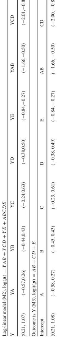
We simulate data from 1000 subjects, on six binary variables {Y,A,B,C,D,E}. Probabilities that correspond to the cells of the 26contingency table are generated in accordance with the log-linear model, log(μ)=Y A B+Y C D+Y E. Adopting the notation inAgresti(2002), a single letter denotes the presence of a main effect, two letter terms denote the presence of the implied first-order interaction and so on and so forth. The presence of an interaction between a set of variables implies the presence of all lower-order interactions plus main effects for that set. Cell counts are simulated according to the generated cell probabilities. Parameter values and the design matrix of the log-linear model used to generate the cell probabilities are given in Supplemental material, Section S2.
We fit to the simulated data the log-linear model,
According to the discussion and results in Sects.1and3, the corresponding logistic regression whereYis treated as the outcome only contains the first-order interactions
A BandC Dplus the main effect forE,
logit(p)= A B+C D+E. (M3)
In Table1, we present credible intervals (CIs) for the parameters of (M3) and the relevant parameters of (M2). The CIs for the corresponding λ andβ parameters are almost identical, considering simulation error. For example, the CI forλY C D1,1,1 is (−2.01,−0.85), whilst the CI forβ1C D,1 is(−2.00,−0.84).
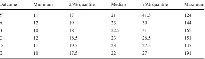
In Table2, we present minimum, maximum and quantile values for theti
observa-tions, for the logistic regression in Table1. It is clear that the simulated data do not represent balanced Binomial experiments whereti = ¯t. The credible intervals listed
in Table 1 demonstrate that the correspondence studied in this manuscript is very robust to departures fromti = ¯t. This is also demonstrated in the real data analysis
presented in the next subsection, where the collected data do not represent balanced Binomial experiments when one of the factors is treated as the outcome. In Sup-plemental material, we present additional analyses on simulated data sets, including results on smaller samples, roughly one quarter the size of the data set analysed in this section. Inferences on the correspondence between the posterior distributions remain unchanged.
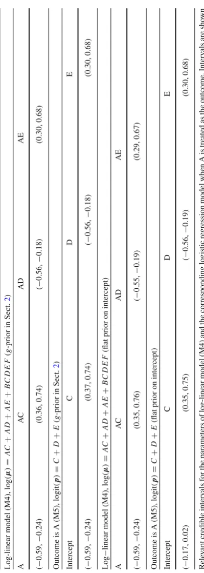
4.2 A real data illustration
Edwards and Havránek(1985) presented a 26contingency table in which 1841 men were cross-classified by six binary risk factors{A,B,C,D,E,F}for coronary heart disease. The data were also analysed inDellaportas and Forster(1999), where the top hierarchical model was, log(μ)= AC+A D+AE+BC+C E +D E+F, with posterior model probability 0.28. In Table3, we present CIs for the parameters of the log-linear model,
AC+A D+AE+BC D E F. (M4) We also present CIs for the parameters of the corresponding logistic regression model when Ais treated as the outcome,
logit(p)=C+D+E. (M5)
Table 2 Simulated data illustration
Outcome Minimum 25% quantile Median 75% quantile Maximum
Y 11 17 21 41.5 124
A 12 19 23 30 144
B 10 18 22.5 31 165
C 12 18.5 23 26.5 151
D 11 19.5 23 27.5 147
E 10 17.5 22 27 191
Maximum, minimum, and quantiles forti,i=1, . . . ,nlt, for different outcomes for the simulated data in
Sect.4.1
coefficients ofC,DandEin the logistic regression model are almost identical to the corresponding CIs forAC,A DandAEin the log-linear model, with differences due to simulation error.
5 Discussion
The correspondence we investigated is not unexpected, given the results inAgresti
(2002) discussed in Introduction, and also the link between theg-prior and Fisher’s information matrix (Held et al. 2015), although this link is stronger for general linear models. Our investigation is also related to Consonni and Veronese (2008), where specifying a prior for the parameters of one model, and then, transferring this speci-fication to the parameters of another is discussed. Of the four strategies considered in
Consonni and Veronese(2008), the one directly linked to our manuscript is ‘Marginal-ization’, as the derived prior for the parameters of the logistic regression is the one that is the marginal prior of the relevant parameters of the log-linear model. Results on the relation between different statistical models are of interest, as they improve understanding and enhance the models’ utility. Often, developments for one mod-elling framework are not readily available for the other. For example,Papathomas and Richardson(2016) comment on the relation between log-linear modelling and vari-able selection within clustering, in particular with regard to marginal independence, without examining logistic regression models.
Our numerical illustrations concern the g-prior, where the parameter g is fixed. To further explore the correspondence between the two modelling frameworks, we also considered the two hyper priors that are prominent inLiang et al.(2008). This is the Zellner–Siow prior [IG(0.5, N/2)], and the prior introduced in the aforementioned manuscript in Sect.4.2, with the suggested specificationα=3. Furthermore, the two data sets were analysed after adopting a mixture ofg-priors such that,g∼IG(ag,bg).
We consideredag =2+mean(g)2/var(g)andbg =mean(g)+mean(g)3/var(g),
affects to a small, but noticeable degree, the posterior credible intervals for the model parameters. For more details, see the analyses presented in Supplemental material.
Theoretical results in this manuscript refer to a specific log-linear model and the corresponding logistic regression model, for a given set of covariates. Therefore, our results should not be misinterpreted as licence to readily translate log-linear model selection inferences to inferences concerning logistic regression models. When per-forming model selection in a space of log-linear models, the prominent log-linear model describes a certain dependence structure between the categorical factors, includ-ing the relation of the binary Y with all other factors. The logistic regression that corresponds to the prominent log-linear model describes the dependence structure between Y and the other factors that is supported by the data in accordance with the log-linear analysis. Therefore, under reasonable expectation, results from a single log-linear model determination analysis may translate, at the very least, to interesting logistic regressions for any of the binary factors that formed the contingency table. However, the mapping between log-linear and logistic regression model spaces is not bijective. Furthermore, posterior model probabilities depend on the prior on the model space, with various different approaches for defining such a prior discussed inDellaportas et al.(2012). For the simulated data analysed in Sect.4.1, log-linear modelY A B+Y C D+Y Ehas posterior probability 0.98, whilst the posterior prob-ability of the corresponding logistic regression model (M3) is 0.59. Similar results from analysing the real data in Sect.4.2, not presented here, also support this note of caution. In all model determination analyses, the Reversible Jump MCMC algorithm proposed inPapathomas et al.(2011) was employed. All possible graphical log-linear models were assumed equally likely a priori, as were all possible logistic graphical models for some given outcome.
Acknowledgements The author wishes to thank Professor Petros Dellaportas and Dr. Antony Overstall
for useful discussions during the preparation of this manuscript. We would also like to thank two reviewers and the editors for comments that helped to improve the manuscript.
Open Access This article is distributed under the terms of the Creative Commons Attribution 4.0
Interna-tional License (http://creativecommons.org/licenses/by/4.0/), which permits unrestricted use, distribution, and reproduction in any medium, provided you give appropriate credit to the original author(s) and the source, provide a link to the Creative Commons license, and indicate if changes were made.
Appendix
Proof of Theorem 1 To facilitate the proof, the following notation is introduced. Using the incidence matrixT discussed in Sect.1, write the mapping betweenβ andλas
β=Tλ, where
T =
⎛ ⎜ ⎝
λ(1) ...
λ(nλY)
⎞ ⎟ ⎠,
superscript. This is a more rigorous definition ofTcompared to the more descriptive definition in Sect.1. To ease algebraic calculations, and without any loss of generality, rearrange the columns ofλ, creating a new vectorλr, so thatTchanges accordingly
to, Tr =
I 0,where I is annβ ×nβ identity matrix andnβ is the number of elements inβ. The rows and columns ofXllare also rearranged accordingly to create
Xrll, so that,
Xrll =
Xlt∗ Xll-lt
0 Xll-lt
(2)
Xll-lt is a square(nll/2×nll/2)matrix. This is because we consider the log-linear
model that, in addition to the terms that involveY, contains all possible interaction terms between the categorical factors inP\{Y}. The number of parameters that cor-respond to the intercept, main effects and interactions forP\{Y}isnll/2.
Denote with j1=2 the number of levels of the binary factorY that becomes the outcome in the logistic regression model. With j2to jq,1≤ q ≤ P−1 denote the
number of levels of the q −1 factors that are present in the log-linear model but disappear from the logistic regression model as they do not interact withY. Then, nll =2× j2× · · · × jq×nlt. Whenq =1, all factors other thanY remain in the
logistic regression model as covariates. Whenq =P−1, the corresponding logistic regression model only contains the intercept. For instance, for a 2Pcontingency table, nll = 2q ×nlt, and forq = 1,nll = 2×nlt. Furthermore, Xlt∗ is anll/2×nβ
matrix. By rearranging the rows of Xrll when necessary, we can writeXlt∗ as Xlt∗ =
(XltXlt. . .Xlt), whereXltis repeated(j1−1)×j2× · · · ×jqtimes. For example,
forq =1,X∗lt =Xlt. Forq =2,Xlt repeats j2times withinXlt∗.
We can now write β = Trλr. For example, assume the log-linear model (M1)
describes a 3×2×2 contingency table. Then,q =1, and the standard arrangement of the elements ofλwould be such that,
Xll =
⎛ ⎜ ⎜ ⎜ ⎜ ⎜ ⎜ ⎜ ⎜ ⎜ ⎜ ⎜ ⎜ ⎜ ⎜ ⎜ ⎜ ⎜ ⎜ ⎝
1 0 0 0 0 0 0 0 0 0
1 1 0 0 0 0 0 0 0 0
1 0 1 0 0 0 0 0 0 0
1 0 0 1 0 0 0 0 0 0
1 1 0 1 0 1 0 0 0 0
1 0 1 1 0 0 1 0 0 0
1 0 0 0 1 0 0 0 0 0
1 1 0 0 1 0 0 1 0 0
1 0 1 0 1 0 0 0 1 0
1 0 0 1 1 0 0 0 0 1
1 1 0 1 1 1 0 1 0 1
1 0 1 1 1 0 1 0 1 1
⎞ ⎟ ⎟ ⎟ ⎟ ⎟ ⎟ ⎟ ⎟ ⎟ ⎟ ⎟ ⎟ ⎟ ⎟ ⎟ ⎟ ⎟ ⎟ ⎠
, λ= ⎛ ⎜ ⎜ ⎜ ⎜ ⎜ ⎜ ⎜ ⎜ ⎜ ⎜ ⎜ ⎜ ⎜ ⎜ ⎜ ⎜ ⎜ ⎜ ⎝ λ λX 1 λX 2 λY 1 λZ 1 λX Y
11 λX Y
21 λX Z
11 λX Z
21 λY Z
11 ⎞ ⎟ ⎟ ⎟ ⎟ ⎟ ⎟ ⎟ ⎟ ⎟ ⎟ ⎟ ⎟ ⎟ ⎟ ⎟ ⎟ ⎟ ⎟ ⎠ , T = ⎛ ⎜ ⎜ ⎝
0 0 0 1 0 0 0 0 0 0
0 0 0 0 0 1 0 0 0 0
0 0 0 0 0 0 1 0 0 0
0 0 0 0 0 0 0 0 0 1
After rearranging,
Xrll=
⎛ ⎜ ⎜ ⎜ ⎜ ⎜ ⎜ ⎜ ⎜ ⎜ ⎜ ⎜ ⎜ ⎜ ⎜ ⎜ ⎜ ⎜ ⎜ ⎝
1 0 0 0 1 0 0 0 0 0
1 1 0 0 1 1 0 0 0 0
1 0 1 0 1 0 1 0 0 0
1 0 0 1 1 0 0 1 0 0
1 1 0 1 1 1 0 1 1 0
1 0 1 1 1 0 1 1 0 1
0 0 0 0 1 0 0 0 0 0
0 0 0 0 1 1 0 0 0 0
0 0 0 0 1 0 1 0 0 0
0 0 0 0 1 0 0 1 0 0
0 0 0 0 1 1 0 1 1 0
0 0 0 0 1 0 1 1 0 1
⎞ ⎟ ⎟ ⎟ ⎟ ⎟ ⎟ ⎟ ⎟ ⎟ ⎟ ⎟ ⎟ ⎟ ⎟ ⎟ ⎟ ⎟ ⎟ ⎠
, λr =
⎛ ⎜ ⎜ ⎜ ⎜ ⎜ ⎜ ⎜ ⎜ ⎜ ⎜ ⎜ ⎜ ⎜ ⎜ ⎜ ⎜ ⎜ ⎜ ⎝ λY 1 λX Y
11 λX Y
21 λY Z
11 λ λX 1 λX 2 λZ 1 λX Z
11 λX Z
21 ⎞ ⎟ ⎟ ⎟ ⎟ ⎟ ⎟ ⎟ ⎟ ⎟ ⎟ ⎟ ⎟ ⎟ ⎟ ⎟ ⎟ ⎟ ⎟ ⎠ ,
Tr =
⎛ ⎜ ⎜ ⎝
1 0 0 0 0 0 0 0 0 0
0 1 0 0 0 0 0 0 0 0
0 0 1 0 0 0 0 0 0 0
0 0 0 1 0 0 0 0 0 0
⎞ ⎟ ⎟ ⎠
For another example, whereq =2, consider again model (M1) but now assume that the interactionY Zis not present in the log-linear model. Then, the Zfactor will disappear from the corresponding logistic regression model, and after rearranging,
Xrll =
⎛ ⎜ ⎜ ⎜ ⎜ ⎜ ⎜ ⎜ ⎜ ⎜ ⎜ ⎜ ⎜ ⎜ ⎜ ⎜ ⎜ ⎜ ⎜ ⎝
1 0 0 1 0 0 0 0 0
1 1 0 1 1 0 0 0 0
1 0 1 1 0 1 0 0 0
1 0 0 1 0 0 1 0 0
1 1 0 1 1 0 1 1 0
1 0 1 1 0 1 1 0 1
0 0 0 1 0 0 0 0 0
0 0 0 1 1 0 0 0 0
0 0 0 1 0 1 0 0 0
0 0 0 1 0 0 1 0 0
0 0 0 1 1 0 1 1 0
0 0 0 1 0 1 1 0 1
⎞ ⎟ ⎟ ⎟ ⎟ ⎟ ⎟ ⎟ ⎟ ⎟ ⎟ ⎟ ⎟ ⎟ ⎟ ⎟ ⎟ ⎟ ⎟ ⎠
, λr =
⎛ ⎜ ⎜ ⎜ ⎜ ⎜ ⎜ ⎜ ⎜ ⎜ ⎜ ⎜ ⎜ ⎜ ⎜ ⎜ ⎜ ⎝ λY 1 λX Y
11 λX Y
21 λ λX 1 λX 2 λZ 1 λX Z
11 λX Z
21 ⎞ ⎟ ⎟ ⎟ ⎟ ⎟ ⎟ ⎟ ⎟ ⎟ ⎟ ⎟ ⎟ ⎟ ⎟ ⎟ ⎟ ⎠ ,
Tr =
⎛
⎝10 01 00 00 00 00 00 00 00
0 0 1 0 0 0 0 0 0
⎞ ⎠
Theg-prior,
λ∼N(mλ,gΣλ)≡N
(log(n¯),0, . . . ,0),gnll XllXll
translates to,
λr ∼N(mλr,gΣλr)≡N
(0, . . . ,0,log(n¯),0, . . . ,0),gnll N X
rllXrll
−1 ,
where log(n¯)is the(nβ+1)th element in the mean vector. Then,
E(β)=E(Trλr)=TrE(λr)=
I 0×μλr =0.
Furthermore,
Var(β)=gTrΣλrTr=
gnll
N Tr X
rllXrll
−1
Tr .
From (2),
XrllXrll
−1 =
Xlt∗Xlt∗ X∗lt Xll-lt
Xll-ltXlt∗ Xll-ltXll-lt+Xll-ltXll-lt
−1
=
Xlt∗Xlt∗ Xlt∗Xll-lt
Xll-ltXlt∗ 2Xll-ltXll-lt
−1 .
From Lutkepohl (1996, p. 147), the submatrixHthat is formed by the firstnβrows and columns of(XrllXrll)−1is,
H = Xlt∗X∗lt
−1
+ Xlt∗X∗lt
−1
Xlt∗Xll-lt
Xll-lt
2I−X∗lt Xlt∗Xlt∗
−1
X∗lt
Xll-lt
−1
×Xll-ltX∗lt Xlt∗Xlt∗
−1
.
Now,Plt ≡Xlt∗(Xlt∗Xlt∗)−1Xlt∗is the projection matrix forX∗lt. It is straightforward
to verify that for a projection matrixPltand a constantc,
(cI−Plt)×
1 cI+
1 c(c−1)Plt
= I.
Therefore,(2I−Plt)=(0.5I+0.5Plt)−1, and consequently,
H = Xlt∗Xlt∗
−1
+ Xlt∗X∗lt
−1
X∗lt Xll-lt
Xll-lt(0.5I+0.5Plt)−1Xll-lt
−1
×Xll-ltXlt∗ Xlt∗Xlt∗ −1
.
Xll-lt is a square matrix of full rank. If Xll-lt was not full rank, then some of its
columns would be linearly dependent. In turn, some of the columns of
Xll-lt
Xll-lt
be linearly dependent, implying the same for columns ofXrll(see Eq.2). This is not
possible asXrll is a design matrix of full rank. Thus,Xll−-1ltexists and,
H = Xlt∗X∗lt
−1
+ Xlt∗X∗lt
−1
X∗lt Xll-lt
X−ll-1lt(0.5I+0.5Plt)X −1 ll-lt
×Xll-ltXlt∗ Xlt∗Xlt∗
−1
= Xlt∗X∗lt
−1
+ Xlt∗X∗lt
−1
X∗lt (0.5I+0.5Plt)Xlt∗ Xlt∗Xlt∗
−1
= Xlt∗X∗lt
−1
+0.5 Xlt∗Xlt∗
−1
+0.5 Xlt∗Xlt∗
−1
=2 Xlt∗X∗lt
−1
=2 j2× · · · × jqXltXlt
−1
Therefore,
Var(β)= gnll N Tr X
rllXrll
−1
Tr
= gnll
N
I 0 XrllXrll
−1I 0
= 2g2j2× · · · × jqnlt
N j2× · · · ×jq
XltXlt
−1
= 4gnlt
N X
ltXlt
−1
Thus,
β∼N
0,4gnlt
N X
ltXlt
−1 ,
which is theg-prior for the parameters of a logistic regression, as described in Sect.2. This completes the proof.
Placing a flat prior on the intercept Assume that a flat prior is placed on the intercept of the log-linear model, after the design matrix has been centred to induce orthogonality between the intercept and the factors that form the contingency table. This does not alter the prior on the parameters of the corresponding logistic regression model. The proof follows along the lines of the proof of Theorem1, if we express the parameters of the logistic regression model asβ=Tr−1λr−1, whereTr−1denotes matrixTr without
the first column with all elements zero, andλr−1 denotes the vector of parameters
λr without the interceptλ. The proof proceeds as above, replacingXrll withXrll−1,
Proof of Theorem 2 The proof utilizes quantities defined earlier in Sect.3and in the proof of Theorem1. First, we will show that, asymptotically, the posterior variance ofβis identical to the posterior variance of the elements ofλthat correspond toβ. Then, we will do the same for the posterior means.
Consider a vector of cell counts n = {n1, . . . ,nll}, and the log-linear model
log(μ)=Xllλ. Then, asymptotically,
Var(λ|n)
g−1Σλ−1+I(λˆ) −1
=
N gnll
XllXll+XllV(λˆ)Xll
−1 ,
whereλˆdenotes the maximum likelihood estimate (MLE). After rearranging the rows and columns of Xll, consider the log-linear model with linear predictor Xrllλr, for
cell countsnr, wherenr isnrearranged to correspond toXrll. Now,
Var(λr|nr)
g−1Σλ−1 r +I λˆr
−1
=
N gnll
XrllXrll+XrllV(λˆr)Xrll
−1
=
Xrll
N gnll +V(
ˆ
λr)
Xrll
−1
= ⎡ ⎢ ⎣ ⎛ ⎝
N
gnllI+V1V2 0
0 gnN
ll +V2 1/2
Xlt∗ Xll-lt
0 Xll-lt
⎞ ⎠
× N
gnllI+V1V2 0
0 gnN
ll +V2 1/2
X∗lt Xll-lt
0 Xll-lt
⎤ ⎥ ⎦
−1
.
V1 denotes a diagonal matrix with nonzero elements exp(X∗lt(i)(Trλˆr)),i =
1, . . . ,nll/2.V2denotes a diagonal matrix with nonzero elements exp(Xll-lt(i)λˆll-lt),
i =1, . . . ,nll/2, whereλˆll-ltdenotes the MLE forλr\Trλr. Now,
Var(λr|nr)
X∗lt A12Xlt∗ Xlt∗A12Xll-lt
Xll-ltA12Xlt∗ Xll-lt(A12+A2)Xll-lt
−1 ,
whereA12= gnN
llI+V1V2andA2=
N
gnllI+V2. From Lutkepohl (1996, p. 147), the submatrixHthat is formed by the firstnβ rows and columns of Var(λr|nr)is,
H = Xlt∗A12X∗lt −1
+ X∗lt A12Xlt∗ −1
×
Xll-lt (A12+A2)Xll-lt −Xll-lt A12Xlt∗ X∗lt A12Xlt∗
−1
Xlt∗A12Xll-lt
−1
×Xll-ltA12Xlt∗ Xlt∗A12X∗lt
−1
= Xlt∗A12X∗lt −1
+ Xlt∗A12X∗lt −1
Xlt∗A12
(A12+A2)−A12Xlt∗ Xlt∗A12Xlt∗ −1
X∗lt A12 −1
×A12Xlt∗ Xlt∗A12X∗lt −1
= Xlt∗A12X∗lt −1
+ Xlt∗A12X∗lt −1
Xlt∗A12
(I+A−121A2)−Xlt∗ X∗lt A12Xlt∗ −1
X∗lt A12 −1
×X∗lt Xlt∗A12X∗lt −1
= Xlt∗A12X∗lt −1
+ Xlt∗A12X∗lt −1
Xlt∗A12
I− I+A−121A2 −1
X∗lt Xlt∗A12X∗lt −1
Xlt∗A12 −1
×X∗lt Xlt∗A12X∗lt −1
.
From Lutkepohl (1996, p. 29, line 6), the expression above simplifies to,
H =
Xlt∗A12X∗lt−Xlt∗A12 I+A−121A2 −1
X∗lt −1
=Xlt∗ A12−A12(I+A−121A2)−1
Xlt∗ −1
.
Within the Bayesian framework, a large sample (N → ∞) will swamp the prior distribution, rendering it irrelevant for deriving posterior inferences (O’Hagan and Forster 2004). This can be viewed as equivalent to considering a flat non-informative prior, in our case assuming thatg → ∞. For a sample size large enough to justify ignoring the contribution of the prior distribution in Var(λ|n), i.e. assuming thatA12=
V1V2andA2=V2, asymptotically,
H
Xlt∗ V1V2−V1V2(I+V1−1V2−1V2)−1
Xlt∗
−1
=Xlt∗V1V2−V12V2(I+V1)−1
Xlt∗
−1
=Xlt∗V1V2(I+V1)−V12V2
(I+V1)−1
X∗lt
−1
=Xlt∗V1V2(I+V1)−1
Xlt∗
−1
=X(V, (I+V, )−1V, +V, + · · · +V,(j1−1)×j2×···×j X −1
V1,reduced denotes a diagonal matrix with elements exp(Xlt(i)(Trλˆr)),i =
1, . . . ,nlt.V2,k,k=1, . . . , (j1−1)×j2× · · · × jq, denotes a diagonal matrix with
elements exp(Xll-lt(nlt(k−1)+i)λˆll-lt). This expression simplifies asqbecomes smaller, i.e. the fewer timesXltis contained withinXlt∗. For example, whenXlt∗ =Xlt, i.e. when
q =1 and all factors other thanY remain in the logistic regression,V1,reduced=V1. We now utilize the standard result (see, for example, Rohatgi 1976, p. 200) that, asymptotically, the Binomial distribution Bin(ti,
exp(Xlt∗(i)(Trλr))
1+exp(X∗lt(i)(Trλr))) of a data point tiyi,i = 1, . . . ,nlt, can be approximated by a Poisson distribution Poisson
(ti
exp(X∗lt(i)(Trλr))
1+exp(Xlt∗(i)(Trλr))). The Binomial observation ti −ti ×yi is formed by adding (j1−1)× j2× · · · × jq independent Poisson cell counts. Considering the Poisson
log-linear model,ti−tiyifollows the Poisson distribution,
Poisson(exp(Xll-lt(i)λˆll-lt)+ · · · +exp(Xll-lt(nlt((j1−1)×j2×···×jq−1)+i)λˆll-lt)). Therefore, approximately,
ti
1
1+exp(Xlt(i)(Trλˆr))
exp(Xll-lt(i)λˆll-lt)+ · · · +exp(Xll-lt(nlt((j1−1)×j2×···×jq−1)+i)λˆll-lt). (3)
In matrix notation, we can now write that, asymptotically,
Var(Trλr|nr)=Tr(Var(λr|nr))Tr
=I 0(Var(λr|nr))
I
0
Xlt tV1,reduced(I+V1,reduced)−2
Xlt
−1
= XltVlogisticXlt
−1 ,
where t is a diagonal matrix with diagonal elements the number of trials ti, and
Vlogistic has diagonal elements tiexp{Xlt(i)βˆ}exp{1 + Xlt(i)βˆ}−2,i = 1, . . . ,nlt.
(XltVlogisticXlt)−1is, asymptotically, the posterior variance of β when the logistic
regression is fitted directly, and thus, we have shown that the posterior variance ofβ is identical to the posterior variance of the elements ofλthat correspond toβ.
We will now show that, asymptotically, the posterior meanE(β|t,y)is the posterior mean of the elements ofλthat correspond toβ. For a sample large enough to justify ignoring the contribution of the prior in (1), we obtain that,E(λ|n)I(λ)ˆ −1I(λ)ˆ λˆ =
ˆ
λ. Similarly, E(β|t,y) ˆβ. Therefore, E(Trλr|n) Trλˆr, and it is sufficient to
show thatβˆ =Trλˆr. Closed-form expressions for the maximum likelihood estimators
model is fitted. SeeWood(2006) for more details. For a linear predictor Xdγ, this
iterative process is based on the formula,
γi t+1=γi t + X
dV(γi t)Xd
−1
XdV(γi t)ζi t.
For a log-linear model,ζi tis denoted byζi tlog-linear, and itsith element,i =1, . . . ,nll,
is,
ζlog-linear(i)=
ni
exp(Xrll(i)λri t)
−1.
For a logistic regression model,ζi t is denoted byζi tlogistic, and itsith element,i = 1, . . . ,nlt, is,
ζlogistic(i)=
tiyi
1+exp(Xltβi t)
−tiexp(Xltβi t)
ti
1+exp(Xltβi t)
exp(Xltβi t)
.
For the log-linear model, the IRLS procedure is written as,
λi t+1
r =λi tr + XrllVlog-linear(λi tr)Xrll
−1
XrllVlog-linear(λi tr )ζi tlog-linear,
where Vlog-linear is a diagonal matrix with diagonal elements exp{Xrll(i)λˆr},i =
1, . . . ,nll. Algebraic operations similar to the ones carried out earlier show that
(XrllVlog-linear(λi t)Xrll)−1partitions as,
⎛ ⎜ ⎜ ⎝
XltVlogisticXlt
−1
−X∗lt V1V2Xlt∗
−1
Xlt∗V1×
V1+I−V1V2Xlt∗
×X∗lt V1V2Xlt∗
−1 X∗lt V1
−1 Xll−-lt1
1 2
⎞ ⎟ ⎟ ⎠,
where1and2are matrices not relevant to this proof. Furthermore,XrllVlog-linear (λi t
r)partitions as,
X∗lt V1V2 0 Xll-ltV1V2 Xll-ltV2
.
For the log-linear model, we writeζlog-linear=(ζ∗lt ζll-lt), whereζ∗ltcorresponds
to the firstnll/2 rows ofXrll. Now, the firstnβelements of(XrllVlog-linear(λi t)Xrll)−1
XltVlogisticXlt
−1
Xlt∗V1V2ζ∗lt−
X∗lt V1V2Xlt∗
−1 Xlt∗V1 ×
V1+I−V1V2Xlt∗ Xlt∗V1V2Xlt∗
−1 X∗lt V1
−1
×V1V2ζlt∗ +V2ζll-lt
.
Theith element ofζ∗lt,i =1, . . . ,nll/2, is,
ζlt(i)=
ni
expXlt(i)Trλi tr
expXll-lt(i)λi tll-lt
−1.
Theith element ofζll-lt,i =1, . . . ,nll/2, is,
ζll-lt(i) =
ti−ni
expXll-lt(i)λi tll-lt
−1.
It is straightforward to show that[V1V2ζ∗lt+V2ζll-lt]is, approximately, a vector of
zeros. To show this, consider, without loss of generality, theith element of this vector,
exp Xlt(i)Trλi tr
exp Xll-lt(i)λi tll-lt
×
ni
expXlt(i)Trλi tr
expXll-lt(i)λi tll-lt
−1
+exp Xll-lt(i)λlli t-lt
×
ti−ni
expXll-lt(i)λi tll-lt
−1
=ti−exp Xll-lt(i)λi tll-lt
×1+exp Xlt(i)Trλi tr
.
Due to the Poisson approximation to the Binomial distribution,
exp Xll-lt(i)λlli t-lt
ti
1
1+expXlt(i)Trλi tr
.
Thus, the elements of vector[V1V2ζlt+V2ζll-lt]are all approximately zero, and the
firstnβelements of(XrllVlog-linear(λi t)Xrll)−1XrllVlog-linear(λi t)ζlog-linearare approx-imately equal to,
XltVlogisticXlt
−1
Xlt∗V1V2ζ∗lt
= XltVlogisticXlt
−1
XltV1,reduced
V2,1. . .V2,(j1−1)×j2×···×jq
Using the Poisson approximation to the Binomial distribution, for theith element of
ζ∗
lt, and assuming without any loss of generality thati<nlt,
ζ∗ lt(i)
ni
expXrll(i)λri t
−1= ni
expXlt(i)Trλri t
ti1+expX1
lt(i)Trλi tr
−1
= ni
1+exp(Xlt(i)Trλi tr)
−tiexp
Xlt(i)Trλri t
tiexp
Xlt(i)Trλri t
.
Thus,
ζ∗
lt(i) 1+exp Xlt(i)Trλri t
−1
ζlogistic(i).
Therefore, the updating step forTrλr is,
Trλi tr+1=Trλi tr + XltVlogisticXlt −1
Xlt
×V1,reduced
I+V1,reduced −1V2
,1. . .V2,(j1−1)×j2×···×jq
ζi t
logistic. . .ζ
i t
logistic
.
=Trλi tr + XltVlogisticXlt −1
Xlt
×V1,reduced
I+V1,reduced −1V2
,1+ · · · +V2,(j1−1)×j2×···×jq
ζi t logistic.
If the logistic regression was to be fitted directly, obtaining the MLE would be based on the IRLS algorithm,
βi t+1=βi t+
XltVlogistic(βi t)Xlt
−1
Xlt×Vlogistic(βi t)ζi tlogistic.
By replacing the sum of the elements of theV2,kmatrices with the approximate
val-ues given in (3), we observe that, asymptotically, the updating step is the same for both
Trλrandβ. Thus, if the starting point forTrλr is the same as the starting point forβ,
the iterative algorithm would give the same MLE for the logistic regression parame-ters and the corresponding log-linear model parameparame-ters. The IRLS algorithm is robust to different starting values when the likelihood is not flat. Therefore, asymptotically,
ˆ
βTrλˆr and the proof is complete.
References
Agresti A (2002) Categorical data analysis, 2nd edn. Wiley, Hoboken
Bapat RB (2011) Graphs and matrices. Springer, Hindustan Book Agency, New Delhi
Consonni G, Veronese P (2008) Compatibility of prior specifications across linear models. Stat Sci 23:232– 353
Dellaportas P, Forster JJ (1999) Markov chain Monte Carlo model determination for hierarchical and graphical log-linear models. Biometrika 86:615–633
Edwards D, Havránek T (1985) A fast procedure for model search in multi-dimensional contingency tables. Biometrika 72:339–351
Fouskakis D, Ntzoufras I, Draper D (2015) Power-expected-posterior priors for variable selection in Gaus-sian linear models. BayeGaus-sian Anal 10:75–107
Held L, Sabanès Bovè D, Gravestock I (2015) Approximate Bayesian model selection with the deviance statistic. Stat Sci.http://www.imstat.org/sts/future_papers.html. Accessed 17 Mar 2016
Kass RE, Wasserman L (1995) A reference Bayesian test for nested hypotheses and its relationship to the Schwarz criterion. J Am Stat Assoc 90:928–934
Liang F, Paulo R, Molina G, Clyde MA, Berger JO (2008) Mixtures ofg-priors for Bayesian variable selection. J Am Stat Assoc 103:410–423
Lutkepohl H (1996) Handbook of matrices. Wiley, Chichester
Mukhopadhyay M, Samantha T (2016) A mixture ofg-priors for variable selection when the number of regressors grows with the sample size. Test. doi:10.1007/s11749-016-0516-0
Ntzoufras I, Dellaportas P, Forster JJ (2003) Bayesian variable and link determination for generalized linear models. J Stat Plan Inference 111:165–180
Ntzoufras I (2009) Bayesian modelling using WinBugs. Wiley, Hoboken
O’Hagan A (1995) Fractional Bayes factors for model comparison. J R Stat Soc Ser B 57:99–138 O’Hagan A, Forster JJ (2004) Bayesian inference, 2nd edn. vol 2B of ‘Kendall’s Advanced Theory of
Statistics’. Arnold, London
Overstall A, King R (2014a) A default prior distribution for contingency tables with dependent factor levels. Stat Methodol 16:90–99
Overstall A, King R (2014b) Conting: an R package for Bayesian analysis of complete and incomplete contingency tables. J Stat Softw 58:1–27
Papathomas M, Richardson S (2016) Exploring dependence between categorical variables: benefits and limitations of using variable selection within Bayesian clustering in relation to log-linear modelling with interaction terms. J Stat Plan Inference 173:47–63
Papathomas M, Dellaportas P, Vasdekis VGS (2011) A novel reversible jump algorithm for generalized linear models. Biometrika 98:231–236
Rohatgi VK (1976) An introduction to probability theory and mathematical statistics. Wiley, New York Sabanès Bovè D, Held L (2011) Hyper-g priors for generalized linear models. Bayesian Anal 6:387–410 Wang X, George GI (2007) Adaptive Bayesian criteria in variable selection for generalized linear models.
Stat Sinica 17:667–690