Using Excel to Explore the Effects of Assumption Violations on One Way Analysis of Variance (ANOVA) Statistical Procedures

(1)

ISSN Online: 2161-7198 ISSN Print: 2161-718X

DOI: 10.4236/ojs.2019.94031 Aug. 13, 2019 458 Open Journal of Statistics

Using Excel to Explore the Effects of

Assumption Violations on One-Way Analysis

of Variance (ANOVA) Statistical Procedures

William Laverty

1*

_{, Ivan Kelly}

2

1_{Department of Mathematics and Statistics, University of Saskatchewan, Saskatoon, Canada}

2_{Professor Emeritus, Department of Educational Psychology & Special Education, University of Saskatchewan, Saskatoon, Canada}

Abstract

To understand any statistical tool requires not only an understanding of the relevant computational procedures but also an awareness of the assumptions upon which the procedures are based, and the effects of violations of these assumptions. In our earlier articles (Laverty, Miket, & Kelly [1]) and (Laverty & Kelly, [2] [3]) we used Microsoft Excel to simulate both a Hidden Markov model and heteroskedastic models showing different realizations of these models and the performance of the techniques for identifying the underlying hidden states using simulated data. The advantage of using Excel is that the simulations are regenerated when the spreadsheet is recalculated allowing the user to observe the performance of the statistical technique under different realizations of the data. In this article we will show how to use Excel to gener-ate data from a one-way ANOVA (Analysis of Variance) model and how the statistical methods behave both when the fundamental assumptions of the model hold and when these assumptions are violated. The purpose of this ar-ticle is to provide tools for individuals to gain an intuitive understanding of these violations using this readily available program.

Keywords

Excel, One-Way ANOVA, Assumption Violations, t-Distribution, Cauchy Distribution

1. Introduction

An important aspect of any statistical procedure is the assumptions that the procedure is based on. For example, using the t-distribution to calculate a 95% confidence interval for the centre of the population that is being sampled

re-How to cite this paper: Laverty, W. and Kelly, I. (2019) Using Excel to Explore the Effects of Assumption Violations on One-Way Analysis of Variance (ANOVA) Statistical Procedures. Open Journal of Statistics, 9, 458-469.

https://doi.org/10.4236/ojs.2019.94031

Received: June 25, 2019 Accepted: August 10, 2019 Published: August 13, 2019

(2)

DOI: 10.4236/ojs.2019.94031 459 Open Journal of Statistics quires that the population being sampled is a normal distribution and that the observations in the sample are independent. If these underlying assumptions do not hold, the desired performance of the statistical procedure may no longer hold true. Sometimes the effect of an invalid assumption on a property of the procedure is minimal, sometimes not so. If the population is non-normal but has a finite mean and variance (such that the Law of Large Numbers and the Central Limit theorem applies), the departure from normality will have little ef-fect on the properties of confidence intervals computed assuming normality when the sample size is adequately large. The reason for this is that it is a conse-quence of the Central Limit Theorem. The purpose of this paper is to show how to use the program Excel to simulate data for which the statistical technique of one-way Analysis of Variance (ANOVA) is used. The advantage of the using the program Excel is that when you press the recalculate button, under the Formulas menu, the data that is generated at random will be regenerated, statistical calcu-lations will be recalculated and relevant graphs will be redrawn. This allows the user to observe the variation in these procedures for different realizations of the data. See Figure 1.

2. A Model for Non-Normality (The Cauchy Distribution, the

t

-Distribution)

For most cases when one-way ANOVA is applicable the normality assumption is appropriate, i.e. the departures of individual observations from their central val-ue are normally distributed. There are however, many examples where this is not the case and extreme departures are more prevalent than predicted by the Nor-mal distribution. This would be dependent on the measurements being collected. For example, if the measurements were measurements of blood pressure, IQ, performance of a political leader one may expect the presence of extreme mea-surements. In such cases an appropriate model of the departures from the cen-tral value would be the t-distribution (a heavy tailed distribution). In this article the reader can use the technique provided to explore the effects of sampling from heavy tailed distributions on ANOVA calculations that assume normality.

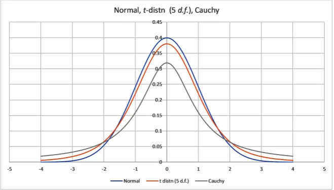
The probability density function of the standard Normal, Students

t-distribution with ν degrees of freedom and the standard Cauchy distribution is given in (1).

( )

(

)

(

)

2 Normal 1 2 ₂ Cauchy ₂ 1 e 2 1 2 : 1 2 1 : 0,1 1 z t f z t f t f x x ν ν ν ν ν ν − + − = +  

Γ_ _{ }_ _

= _ + _

   

Γ _{ }

=   π       π    

π + _

(3)

[image:3.595.219.529.73.203.2]

DOI: 10.4236/ojs.2019.94031 460 Open Journal of Statistics Figure 1. Excel recalculation.

The Standard Cauchy distribution is equivalent to the t distribution with 1 degree of freedom. A graph of the standard normal distribution, the t-distribution with 5 degrees of freedom, and the Cauchy distribution is in Figure 2.

The Cauchy Distribution is an example of a distribution where the Law of Large numbers and the Central limit Theorem do not apply [4]. In order for these two Laws to hold both the mean and higher moments have to exist and be finite. This is not the case for the Cauchy distribution. There is no convergence of the distribution of the sample mean to the central value. In fact the distribu-tion of the sample mean is the Cauchy distribudistribu-tion for any sample size (i.e. the distribution of the sample mean is the same as that of any individual observation when the data comes from the Cauchy distribution). The Cauchy distribution is a heavy-tailed distribution. The t-distribution is also a heavy-tailed distribution (but not as extreme) when the degrees of freedom ν is small. As the degrees of freedom increases the t distribution approaches the standard normal distribu-tion. Tsay [5] uses the t-distribution with 5 degrees to model random distur-bances that appear in various time series models of financial data. This accounts for the sometimes extreme changes that appear in financial data. The Cauchy distribution is appropriate if extreme values are prevalent in the data (the

t-distribution with degrees of freedom higher than 1 in the less extreme case). This could occur in surveys where individuals were asked to make a continuous measurement of some quantity and extreme values were prevalent in the popu-lations. For example, measurements of blood pressure, IQ, and performance of a political leader, could result in non-normal data with extreme values at either end. In such cases alternatives to ANOVA are appropriate.1_{We haven’t} consi-dered these alternatives in this paper.

The t-distribution with ν degrees of freedom can also be shown to be mixture of Normal distributions with mean 0 and variance W, where the weighting dis-tribution for W is the inverse gamma distribution with α = ν/2 and β = ν/2 (Cook [6]). This implies that a random variable T will have the t-distribution with ν degrees of freedom if W is selected from the inverse gamma distribution with α = ν/2 and β = ν/2 and then T is selected from Normal distributions with mean 0 and variance W.

(4)

DOI: 10.4236/ojs.2019.94031 461 Open Journal of Statistics

3. Simulation of Data from a Continuous Distribution in

Excel

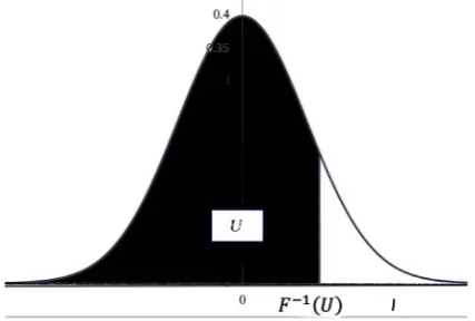
Uniform random variates on [0, 1] can be generated in Excel with the func-tion “RAND()”. The generafunc-tion of random variates from a continuous dis-tribution with measure of central location μ and measure of scale σ, can be carried out using the inverse-transform method (Fishman [7]). Namely Y =

F−1₍_U_{) where}_F₍_u_{) is the desired cumulative distribution of}_Y_and_U_{has a} uniform distribution on [0, 1] (see Figure 3). In Excel this is achieved for the Normal distribution (mean μ, standard deviation σ) with the function “μ + σ* NORMSINV(RAND())” and for the Cauchy (t with 1 d.f.) location parameter,

μ, and scale parameter, σ, “μ + σ* TINV(2*(1-RAND()),1)” (Figure 3). Comment: The Excel function TINV(U,df) does not calculate F−1₍_U_{) for} the t-distn with degrees of freedom df, however the excel function TINV(2*(1-U),df) does achieve the desired calculation.

4. Setting Up the Excel Worksheet to Simulate Anova Data

The data simulated will come from 3 populations (this can easily be genera-lized to more than 3 populations). The parameters of the populations

1) mean (central location), stored in cells C2:E2

2) standard deviation (scale parameter), stored in cells C3:E3 3) sample size), stored in cells C4:E4

4) a parameter that determines normality of the data versus non-normality. stored in cells C1:E1. This parameter is set to zero if the desired data is nor-mal. If this parameter is set to an integer, ν, greater than 0 the data will come from a t -distribution with ν degrees of freedom. The t -distribution is a non-normal heavy-tailed, centered and symmetric about zero.

[image:4.595.209.539.515.703.2]

5) A final parameter (precision), located in cell A2 specifies the of decimal places that the raw data is rounded to (Table 1 below)

(5)

[image:5.595.267.481.73.217.2]

DOI: 10.4236/ojs.2019.94031 462 Open Journal of Statistics Figure 3. Three continuous population distributions (normal, t and Cauchy).

Table 1. Excel worksheet.

A B C D E

precision normality 0 0 0

2 loc. par. 10 10 15

scale par. 3 3 3

n 10 10 10

5. Generating Simulated Data

Copy the observation numbers (1 to 10) in Cells B7:B:16 Paste in cell C7 the formula

=IF($B7>C$4,"",ROUND(C$2+C$3*IF(C$1=0,NORMSINV(RAND()),TINV (2*(1-RAND()),C$1)),$A$2))”

Copy this formula to cells C7:E16. If the normality parameter is 0, the data generated will be from the normal distribution with mean = “loc. Par.” And standard deviation = “scale par.”). If the normality parameter is an integer greater than 0, the data will be a random number with a t-distribution scaled by the “scale par.” and location shifted by the “loc. par.” The data will be rounded to the number of decimals specified by “precision”.

For each population compute Ti = Σx and Σx2. Paste formula “=SUM(C7:C16)” and formula “=SUMSQ(C7:C16)” in cells C18 and C19. Copy these formulae to cells C18:E19.

6. Computation of Statistics Required for One-Way

ANOVA

Suppose we have data from k Normal populations with means

1, , , ,2 3 k

µ µ µ _ µ and common standard deviation σ. Let

{

x iij, =1,2, , ; k j=1,2, , ni

}

denote data from these populations. Let xij = the jth_{observation from the}_ith_population,_n

i = the sample size from the ith population.

Let

1

i

n ij j i

i

x x

n

=

∑

and

(

)

2 1

1

i

n

ij i

j i

i

x x

s

n

= −

=

−

(6)

DOI: 10.4236/ojs.2019.94031 463 Open Journal of Statistics denote the sample mean and standard deviation from the ith_{population. To} compute the sample mean and sample Standard deviation for each population, paste the formulae “=AVERAGE(C7:C16)” and “=STDEV(C7:C16)” in cells C21 and C22. Copy these formulae to cells C21:E22.

To test the null hypothesis H0: µ µ1= 2==µk against HA: µi≠µj for at least one pair i, j we use the test statistic

(

) (

)

(

)

(

)

(

)

(

)

2 . Between 1 2 Within 1 1

1 SS 1

SS i k i i k n ij i i j

x x k k

F

N k

x x N k

= = = − − − = = − − −

∑

∑ ∑

. (3)

where

(

)

2

Between 1 .

SS =

∑

ki= x xi− and

(

)

2 Within 1 1

SS k ni

ij i i= j= x x

=

∑ ∑

− (4)

This statistic has an F-distribution with ν1 = k – 1 degrees of freedom in the numerator and ν2 = N–k degrees of freedom in the denominator.

The computing formulae for

2 2 Between SS i i i T G n N

=

∑

− _and 2 2

Within

SS i

ij

i j i

i T x

n

=

∑ ∑

−

∑

₍₅₎

where

i i ij ij

T =

∑

x =

∑∑

x and G=

∑

iTi=

∑∑

xij (6) The testing for One-way ANOVA is carried out using the Analysis of Va-riance table (Table 2).

Place the formula “=SUM(C18:E18)” in cell G18 to compute the grand to-tal, G=

∑

iTi=

∑∑

xij and the formula “=SUM(C19:E19)” in cell G19 to compute 2_.

ij x

∑∑

Place the formula “=C182_{/C4” in cell C24 and copy to E24 to compute} i2 i T

n for each sample. Then place the formula “=SUM(C24:E24)” in cell G24 to compute i2

i i T

n

∑

.

To compute SSBetween i i2 2 i

T G

n N

=

∑

− place the formula “=G24-G182_{/F4” in}

cell J22 and to compute 2 2 Within

SS i

ij

i j i

i T x

n

=

∑ ∑

−

∑

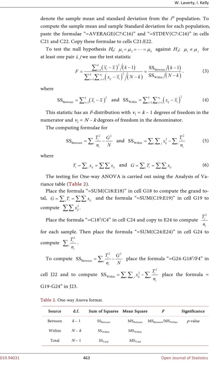
_{place the formula =}

[image:6.595.127.541.43.774.2]

G19-G24” in J23.

Table 2. One-way Anova format.

Source d.f. Sum of Squares Mean Square F Significance

Between k − 1 SSBetween MSBetween MSBetween/MSWithin p-value

Within N − k SSWithin MSWithin

(7)

DOI: 10.4236/ojs.2019.94031 464 Open Journal of Statistics The formulae for degrees of freedom, Mean Square can be placed in the appropriate cells L22:L23 and K22:K23.

The formula for the F statistic “=L22/L23” can be placed in cell M22. The formula for the p-value of the observed F value “=FDIST(M22, K22, K23)” can be placed in cell N22.

The formula for a (1 − α)100% confidence interval for the mean of the ith sample is:

( Error) Error

2

MS

df i

i x t

n

α

± (7)

This formula “=C$21-TINV(0.05,$K$23)*(SQRT($L$23)/$C$4)” can be placed in Cell I28 for the lower limit and in cell I29

“=C$21+TINV(0.05,$K$23)*(SQRT($L$23)/$C$4)” for the upper limit. These formulae can be copied to cells I28:K29 to do the computation for all samples.

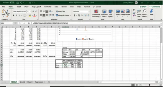
The spreadsheet should now look like Figure 4. To construct Box-whisker plots of the data

1) Select a range containing the data C6:E16 for 10 observations from each sample from the 3 Populations.

2) The menu item for Box-plots can be found under the histogram item (Figure 5).

Figure 4. Spreadsheet of completed one-way Anova.

[image:7.595.232.515.380.532.2]

(8)

DOI: 10.4236/ojs.2019.94031 465 Open Journal of Statistics Comment: There is a problem with Excel’s method of drawing box-plots. If in the data range there is a blank cell, when drawing a box-plot Excel treats that cell as containing a zero rather than treating the observation as non-existent.

7. Exercises That Can Be Performed to Illustrate the

Effects of Assumption Violations on ANOVA

In these exercises we generate samples using different ANOVA assumptions to examine the violations of these assumptions on the ANOVA calculations.

1) Equal means, Equal Standard deviations, Equal sample size, Normality:

μ1 = 10, σ1 = 2, n1 = 10, μ2 = 10, σ2 = 2, n2 = 10, μ3 = 10, σ3 = 2, n3 = 10; normality = 0 (normal distribution)

Comment: When the population means are all equal and the assumptions are satisfied the p-values come from a uniform distribution from 0 to 1. Thus 5% of the time the p-value will be less than or equal to 0.05 resulting in a type I error.

2) Unequal means (H0 false), Equal Standard deviations, Equal sample size, Normality:

μ1 = 15, σ1 = 2, n1 = 10, μ2 = 10, σ2 = 2, n2 = 10, μ3 = 5, σ3 = 2, n3 = 10; nor-mality = 0 (normal distribution)

Anova

Source S.S. d.f. M.S. F pvalue Between 0.183647 2 0.091823 0.020396 0.979826 Within 121.5552 27 4.502046

Total 121.7389 29

(9)

DOI: 10.4236/ojs.2019.94031 466 Open Journal of Statistics Comment: The ability to detect differences among the means will depend

on the non-centrality parameter

(

)

2

i i in µ µ

δ

σ −

=

∑

where i i i

i i n

n

µ µ =

∑

. (Kirk, [8]) The larger the value of the non-centrality parameter, δ, the greater the power of the F-test. (i.e. the greater the probability of picking out existent differences.)

3) Unequal means (H0 false), Equal Standard deviations, Equal sample size, Normality (low non-centrality parameter):

μ1 = 11, σ1 = 5, n1 = 10, μ2 = 10, σ2 = 5, n2 = 10, μ3 = 9, σ3 = 5, n3 = 10; nor-mality = 0 (normal distribution)

Comment: In this case the non-centrality parameter is smaller than the previous example. The p-value of the F-test is considerably higher resulting in an inability to detect a difference in the means.

4) Equal means, Unequal Standard deviations, Equal sample size, Normality:

μ1 = 10, σ1 = 2, n1 = 10, μ2 = 10, σ2 = 5, n2 = 10, μ3 = 10, σ3 = 10, n3 = 10; normality = 0 (normal distribution))

Anova

Source S.S. d.f. M.S. F pvalue Between 614.531 2 307.2655 42.81839 4.22E-09 Within 193.7524 27 7.176017

Total 808.2834 29

pop'n 1 pop'n 2 pop'n 3 lower 15.62 9.20 4.59 upper 16.72 10.30 5.69 95% CONFIDENCE LIMITS

Anova

Total 830.1817 29

(10)

DOI: 10.4236/ojs.2019.94031 467 Open Journal of Statistics Comment: The anova F-test is to some extent robust against the violation of the assumption of the homogeneity of variance (Bathke [9]).

5) Equal means, Equal Standard deviations, Equal sample size, non-Normality:

μ1 = 10, σ1 = 2, n1 = 10, μ2 = 10, σ2 = 2, n2 = 10, μ3 = 10, σ3 = 2, n3 = 10; normality = 1 (Cauchy distribution)

Comment: Recall when the data comes from the Cauchy distribution

Anova

Total 2302.71 29

pop'n 1 pop'n 2 pop'n 3 lower 8.97 7.48 6.22 upper 12.73 11.24 9.98 95% CONFIDENCE LIMITS

Anova

Total 651.0625 29

pop'n 1 pop'n 2 pop'n 3 lower 10.48 9.30 8.55 upper 12.46 11.28 10.54

(11)

DOI: 10.4236/ojs.2019.94031 468 Open Journal of Statistics (t-distribution 1 d.f.) neither the law of large numbers or the Central Limit Theorem are applicable. In fact, the distribution of the sample mean for n

observations is the same as a single observation. This is illustrated in this ex-ample.

8. Discussion

In applying any statistical procedure it is important understanding the assump-tions on which it is based. It is also important to understand the effects on these procedures of the violations of these assumptions. Sometimes the effects of the violations can be extreme, sometimes minimal. The purpose of this article is to provide tools for individuals to gain an intuitive understanding of these viola-tions using the readily available program Microsoft Excel. The advantage of the using the program Excel is that when you press the recalculate button, under the Formulas menu, the data that is generated at random will be regenerated, statis-tical calculations will be recalculated and relevant graphs will be redrawn. The statistical procedure that we have chosen to illustrate these tools is one-way ANOVA. This procedure is an important component of introductory statistical courses and textbooks. The tools can be easily extended to other and more ad-vanced univariate procedures.

9. Conclusion

Excel is a very useful tool for examining the performance of One-Way Anova of variance both when the assumptions hold and more importantly when the as-sumptions are violated.

Conflicts of Interest

The authors declare no conflicts of interest regarding the publication of this pa-per.

References

[1] Laverty, W.H., Miket, M.J. and Kelly, I.W. (2002) Simulation of Hidden Markov Models with EXCEL. Journal of Royal Statistical Society: Series D, 51, 31-40.

https://doi.org/10.1111/1467-9884.00296

[2] Laverty, W.H. and Kelly, I.W. (2018) Using Excel to Simulate and Visualize Condi-tional Heteroskedastic Models. American Journal of Theoretical and Applied Statis-tics, 7, 242-246.

[3] Laverty, W.H. and Kelly, I.W. (2019) Using Excel to Visualize State Identification in Hidden Markov Models Using the Forward and Backward Algorithms. Applied Mathematical Sciences, 13, 151-162.https://doi.org/10.12988/ams.2019.812195

[4] Feller, W. (1971) An Introduction to Probability Theory and Its Applications, Vo-lume II. 2nd Edition, John Wiley & Sons Inc., New York.

[5] Tsay, R.S. (2010) Analysis of Financial Time Series. 3rd Edition, Wiley, Hoboken.

https://doi.org/10.1002/9780470644560

(12)

DOI: 10.4236/ojs.2019.94031 469 Open Journal of Statistics https://statisticaloddsandends.wordpress.com/2018/03/03/t-distribution-as-a-mixtu

re-of-normals/

[7] Fishman, G.S. (1995) Monte Carlo, Concepts, Algorithms and Applications. Sprin-ger, Berlin.

[8] Kirk, R. (2012) Experimental Design: Procedures for Behavioral Sciences. Sage Pub-lications, Thousand Oaks. https://doi.org/10.4135/9781483384733