Multi-component Decomposition of Astronomical Spectra by Compressed Sensing
Mark C. M. Cheung1,2 , Bart De Pontieu1,3,4 , Juan Martínez-Sykora1,5 , Paola Testa6 , Amy R. Winebarger7 , Adrian Daw8 , Viggo Hansteen1,3,4 , Patrick Antolin9 , Theodore D. Tarbell1 , Jean-Pierre Wuelser1, and Peter Young8,10
The MUSE Team
1
Lockheed Martin Solar & Astrophysics Laboratory, 3251 Hanover Street, Palo Alto, CA 94304, USA;[email protected]
2
Hansen Experimental Physics Laboratory, Stanford University 452 Lomita Mall, Stanford, CA 94305, USA
3Rosseland Centre for Solar Physics, University of Oslo, P.O. Box 1029 Blindern, NO-0315 Oslo, Norway 4
Institute of Theoretical Astrophysics, University of Oslo, P.O. Box 1029 Blindern, NO-0315 Oslo, Norway
5
Bay Area Environmental Research Institute, NASA Research Park, Moffett Field, CA 94035, USA
6
Harvard-Smithsonian Center for Astrophysics, 60 Garden Street, Cambridge, MA 02193, USA
7
NASA Marshall Space Flight Center, Huntsville, AL 35812, USA
8
NASA Goddard Space Flight Center, Greenbelt, MD 20771, USA
9
School of Mathematics and Statistics, University of St. Andrews, St. Andrews, Fife KY16 9SS, UK
10
Northumbria University, Newcastle Upon Tyne, NE1 8ST, UK
Received 2019 February 1; revised 2019 May 17; accepted 2019 May 18; published 2019 August 27
Abstract
The signal measured by an astronomical spectrometer may be due to radiation from a multi-component mixture of plasmas with a range of physical properties (e.g., temperature, Doppler velocity). Confusion between multiple components may be exacerbated if the spectrometer sensor is illuminated by overlapping spectra dispersed from different slits, with each slit being exposed to radiation from a different portion of an extended astrophysical object. We use a compressed sensing method to robustly retrieve the different components. This method can be adopted for a variety of spectrometer configurations, including single-slit, multi-slit (e.g., the proposed MUlti-slit Solar Explorer mission), and slot spectrometers(which produce overlappograms).
Key words:instrumentation: spectrographs– line: profiles–methods: observational–Sun: corona –techniques: imaging spectroscopy
1. Introduction
From solar flares to quasars, spectrometers are used to investigate a wide variety of astrophysical phenomena. To obtain measurements of the physical conditions of the emitting material (e.g., extreme UV emission lines of many-times ionized Fe atoms)inevitably requires a forward model with the following components:
1. P—A physics-based model of the radiative process
operating in the astrophysical object of interest (e.g., emission, absorption, scattering, and gravitational redshift);
2. O—An optical model of the telescope (including the
point-spread function(PSF), instrumental spectral broad-ening, and if the telescope is ground-based, atmospheric seeing); and
3. D—A detector model capturing the properties of the
sensing system (e.g., nonlinearity, dark current, gain patterns, and sources of noise).
The goal of spectroscopic measurements is to provide observational constraints of the physical properties of the system. For the sake of discussion, suppose one has perfect knowledge of the optical system and the detector. Even then, a physics model is still required for the most basic of spectro-scopic measurements, such as the Doppler shift of a spectral line. For instance, consider spectroscopic measurements of extreme UV(EUV)emission lines from solar coronal plasma in the optically thin regime in the absence of scattering. In order
to extract the Doppler shift of the line, the local enhancement
(emission line) or deficit (absorption line) in the detected spectrum must first be associated with a known spectral line from a certain atomic species. This provides a reference rest wavelength of the line against which a Doppler shift (in wavelength and in velocity)can be measured. Accounting for, or in the absence of, gravitational redshift, the Doppler shift informs us about the motion of plasma along the line of sight
(LOS), vLOS. Given an atomic model(e.g., CHIANTI, Dere
et al. 1997; Young & Landi 2009; Landi et al.2013)we can also attribute the emission line to plasma in a certain range of temperatures. Assuming thermal equilibrium conditions (e.g., thermal collisional excitation rates balanced by spontaneous radiative deexcitation), the atomic model also provides the thermal widthσthof the line.
In the general case, the spectrum measured at the detector may be due to a heterogeneous mixture of plasmas at different temperatures and Doppler velocities. For example, measure-ment of a spectral line with an observed width σobs>σth suggests the emitting plasma has multiple components moving at different LOS velocities (which, depending on the physics model, may be interpreted as a sign of turbulence; Brooks & Warren2016; van Ballegooijen et al.2017; Polito et al.2018). The detection of multiple spectral lines associated with different temperatures suggests multiple thermal components in the emitting plasma. The presence of multiple components contributing to a single spectrum on the detector may be due to spatial inhomogeneities along the LOS or within the plane-of-sky area visible to the slit (or multiple slits in the case of a multi-slit instrument).
The aim of this work is to describe a method for decomposition of the spectra into constituent components of
© 2019. The American Astronomical Society.
the emitting spectra by techniques of compressed sensing. The driver behind this work is to address the complexities introduced by the use of multi-slit instrumentation in solar physics(e.g., the Multi-slit Solar Explorer or MUSE, proposed as a NASA Heliophysics mission), which promises to greatly increase the field of view and/or drastically improve the temporal cadence of spectroscopic data. In this paper, the method is demonstrated in the context of MUSE, for which the goal is to account for any effect of blends on the primary lines of interest, rather than to use the decomposition results directly. However, the method described is very general and can be applied to a host of other astrophysical problems. The article is structured as follows. Section2gives a mathematical description of the problem for the general case. Section 3 briefly discusses the parameter space we explore. Section 4 describes in some detail the compressed sensing approach, while Section5discusses some examples of application of the method to solar spectral data. Finally, in Section 6we discuss the presented method and its results.
2. Problem Statement
Consider a multi-slit sensing system with a set of parallel slits S={Sm; m= ¼0, ,M -1}, each of width w, and a common detector at the focal plane(see Figure1). Assume the regular slit spacing dlf A, where λis the wavelength of
observation andf/Ais the f-ratio of the light beam at the slit
(fandAbeing the effective focal length and aperture diameter, respectively, of the telescope that feeds the spectrograph).
The detector has a 2D array of pixels indexed[i,j], and we assume that icorresponds precisely to the spectral dimension andjcorresponds precisely to the spatial dimension along the slit, as can be accomplished through geometric corrections when instrument alignment is not perfect. Variations along i and j are therefore separable, and we need only to consider variations in i for the decomposition. The measured spectro-gramy[i](intensity at theith pixel)can have contributions from photons originating from multiple slits.
= S =- Y
D O P
y i[ ] ( mM 01 m( ( ))[ ])i , ( )1
whereOm(P(Ψ))[i]is the spectrogram due solely to radiation from slitm. The emitting material seen by slit mhas a density function Ψ over some parameter space of physical properties
[image:2.612.122.494.58.358.2](e.g., temperature, density, and Doppler velocity)and radiates a spectrum denotedIλ=P(Ψ). The operatorOmacting onP(Ψ) represents how the radiation is processed by the optical system, including how light through an individual slit is dispersed and focused onto the detector to form a spectrum. For two adjacent identical slits that happen to observe the same packet of material residing in the astrophysical object of interest with physical propertyΨwould lead to the same spectrumO(P(Ψ)),
exceptOm+1( ( ))P Y would be translated fromOm+1( ( ))P Y by some pixel offset Δi, namely
Y = Y + D
+
Om 1( ( ))[ ]P i O Pm( ( ))[i i]. ( )2
For an ideal detector, the operator D gives an identity mapping (i.e., it preserves the spectrograph exactly). A noisy, linear detector can be described asD y( )=Gy+e, whereGis the gain andeis the stochastic(and perhaps systematic)noise introduced by the detector.
In general, different slits will be exposed to incident radiation from different parts of the astrophysical scenery. So the challenge is to decompose the net measured spectrum y[i] into constituent components by identifying
1. the slit(s)that contributed to the net spectrogram, and 2. the physical properties of the radiating material along the
column of integration in the LOS seen by each slit. Though the above description of the problem applies to both radiation from optically thick and optically thin plasmas, the rest of this paper will be concerned with the simple case of optically thin plasmas. This allows us to express the physical modelP as a linear operator over the parameter space density function Ψ. The aim of measuring the physical properties of emitting material is equivalent to finding the function Ψ such that Equation (1) is satisfied. The following sections (in particular Section5)will provide some concrete examples.
3. Parameter Spaces
3.1. Differential Emission Measure(DEM)
A common concept encountered in EUV and X-ray observations of solar plasma is the DEM(see, e.g., Boerner et al.2012), defined by the relation
ò
=y i K T DEMT dT, 3
T T i 0 1 [ ] ( ) ( ) ( )
where y[i]is the detected spectrogram (after dark subtraction, flatfielding, correction for nonlinearities, etc.), Ki(T) is the temperature response function of the ith spectral channel, and DEM ( )T dT=
ò
0¥ n T dle( )2 is the electron density squared, integrated along the LOS, contained in a temperature bin of width dT. Ki(T) encapsulates assumptions about the radiative properties of the emitting plasma (i.e., P) and the optical properties of the system (i.e., O), such as PSF, effective area, etc.The aim of the DEM inversion problem in previous work was to recover DEM(T)given a set of measurementsy[i](see Cheung et al. 2015, and references therein). In that context, DEM(T) is the parameter space density function Ψ, which spans over the temperature range[T0,T1], but did not include
the dimensions of Doppler velocity, as we assumed that the observing system in question(e.g., the EUV channels of the Atmospheric Imaging Assembly (AIA), see Boerner et al. 2012; Lemen et al. 2012) does not have sufficient spectral resolution to resolve Doppler shifts. Furthermore, the physical model of radiation assumes the emissivity of EUV spectral lines is only a function of T (though as shown by Martínez-Sykora et al. 2011; Testa et al. 2012, there is also a slight dependence on plasma density).
3.2. Velocity DEM(VDEM)
As an extension of the DEM inversion problem, consider the situation where the sensing system has sufficient spectral resolution and sampling to be sensitive to Doppler shifts. In this case the parameter space density function Ψ(T, v) spans temperature and Doppler velocity space. Solving the VDEM problem means we seek to quantify how much plasma(in terms of emission measurene2)is at a certain temperatureT moving
with Doppler velocityv. In other words,findΨ(T,v)such that the following relation holds:
ò ò
= Y
y i K T v, T v dTdv, . 4
v v T T i 0 1 0 1 [ ] ( ) ( ) ( )
In the case of multiple slits, the rhs of Equation (4) also includes a sum overm(the index for the M slits)andKi,mmay
be slit-dependent. In Section4, we describe how a compressed sensing technique is used for the class of problems similar to Equation(4).
4. Compressed Sensing Solution Approach
Suppose Ψ 0 is a density function over an n-dimen-sional parameter space f=(f f f0, 1, j,...,fn-1), where
fjÎ[fj,0,fj,1], and fj,0 and fj,1 are the lower and upper
bounds of the jth parameter. The operator P acts on f to generate (and propagate) radiation to the sensing system. The operator O takes this incident radiation arriving at the sensing system(e.g., a telescope and its optical system)and produces the M-tuple y (each component of y is the spectrogram measured in a pixel of the detector). P and
O,and the deterministic part ofD(e.g., gain)are assumed to be known.
The solution strategy begins with generating response functions. Consider each dimension of parameter space is discretized into afinite number of pointsNj. For each pointfin
parameter space, compute the detector responserfaccording to Equation (1). The set of all response vectors are used to generate the response matrix R=( )rf . R has dimensions N×M, where N= Pnj=-01Nj. Parameter estimation (i.e., measuring the physical properties of the radiating plasma) is then equivalent to solving the following linear system forx
=
y Rx, ( )5
where x=( )xj ,xj0 is an N-tuple of coefficients for the response functions. In other words, we seek to express the measured spectrogram yas a linear superposition of response functions rf. For a multi-dimensional parameter space, this linear system may be underdetermined. There are a variety of compressed sensing schemes that can be used to tackle such types of problems. For instance, for DEM reconstruction from narrowband EUV data taken by the AIA(Boerner et al.2012; Lemen et al. 2012) on board NASA’s Solar Dynamics Observatory(SDO; Pesnell et al.2012), Cheung et al. (2015) presented a validated inversion scheme based on basis pursuit
(Chen et al. 2001). That particular problem has M=6 (six EUV channels used)and N≈20(number oflogT bins). For much larger problem sizes, we found the lasso method
seeks a solution for Equation(5)byfinding:
a
= - +
#
x argmin 1 y Rx x
2 , 6
2
1 ⎡
⎣⎢ ( ) ∣ ∣⎤⎦⎥ ( )
where∣ ∣x1= SiN=-01∣ ∣xi is the L1 norm ofx. In other words,x# is the argumentxwhich minimizes the objective function in the square brackets. By adding an L1 penalty term, Lasso promotes sparsity in the solution.αis a hyperparameter(i.e., a parameter that is notfitted by the algorithm)used to control the level of sparsity. A larger value ofαtends to yield solutions that have smaller L1 norm(more sparse).
5. Examples of Spectral Sensing Systems
5.1. Single-slit Spectrometer:Hinode/EIS
Perhaps the most common type of astronomical spectrometer instruments are those with a single slit,i.e.,M=1. An example is the EUV Imaging Spectrometer(EIS; Culhane et al.2007)on board theHinodemission(Kosugi et al.2007).
Hinode/EIS is sensitive to emission lines of many-times
ionized metallic species (e.g., Fe, O, and Ni) found in solar coronal plasmas at temperatures between logT K~5.0 and logT K~7.3.
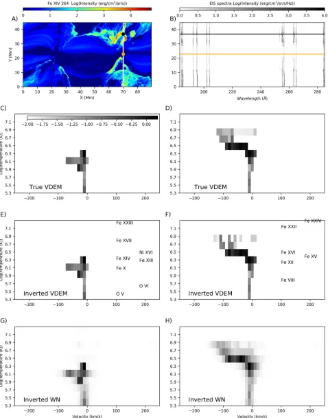
In general, an EIS spectrogram consists of multiple emission lines corresponding to different plasma components of various temperatures and Doppler velocities. Sample spectrograms are shown in Figure2. Using a snapshot from a three-dimensional radiative MHD simulation of a solarflare(Cheung et al.2019), we synthesized the optically thin emergent EUV radiation using atomic models from the CHIANTI database (version 8 Del Zanna et al.2015). A spatial intensity image of the FeXIV 264Åline is shown in panel(A)of Figure2. Panel(B)of the same figure shows the spectrogram if the EIS slit were placed along the vertical line(x=70 Mm)in panel(A). Along the EIS slit, we sample VDEMs from two positions indicated by the colored dots in panel (A) and the corresponding colored horizontal lines in panel(B). The ground truth VDEMs(i.e., as sampled from the MHD simulation)at these two positions(in order of increasingycoordinate position)are shown in panels
(C)and(D)respectively.
To invert the spectrograms for VDEMs, we follow the procedure outlined in Section 4. Consider a unit of emission measure (e.g., for observations of solar plasmas at 1 au, an emission measure of EM0=1025cm−5or above is generally detectable given a sufficiently bright emission line and sufficient effective area and exposure time). Consider a VDEM distributionΨ(T,v)=EM0δ(T0,v0), i.e., an isothermal plasma
at temperature T0 at a single LOS velocity v0. Using the
physical modelP(CHIANTI)and instrumental response model O
( ), compute the response vector r(T v0, 0) for this VDEM distribution, and repeat for other values ofT0andv0in VDEM
space. This allows us to construct the response matrix Rused for VDEM inversions. The parameter space has a velocity range of±400 km s−1with a velocity bin size of 10 km s−1and the temperature ranges fromlog( [ ])T K =5.3tolog( [ ])T K = 7.3 with a bin size of 0.2. i.e., N=80×9=720. For the radiation model(i.e.,P)we consider plasma with solar coronal abundances. The emission model includes 18 spectral lines
(from Doschek et al.2013)which are listed in panels(E)and
(F) of Figure 2, and cover a broad temperature range from ~
T
log( max[ ])K 5.45 (OV248.46Å), to log(Tmax[ ])K ~7.2
(FeXXIV 255.1Å). The detector model D includes photon
noise, based on Poisson distribution and exposure times of 30 s, using the EIS effective area. Panels (E) and (F) show the VDEM distributions inverted from the spectrogram displayed in panel(B), while panels(G)and(H)show the average of the inverted VDEMs over 250 realizations of the photon noise. Although there are imperfections in the recovered VDEM, they reproduce the salient features in the ground truth VDEMs. Over a range of temperatures, the inversion correctly reproduces the spread of emission measure in Doppler velocity space. For instance, the range of Doppler velocities with significant emission measure is much narrower forlogT[ ]K <6.
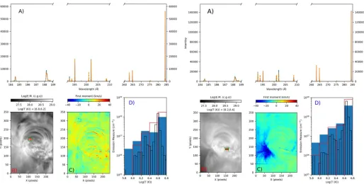
We also tested our VDEM inversion method on actual Hinode/EIS observations. Even though in this case the ground truth is unknown, we have confirmed that the results we obtain are in good agreement with findings of previous detailed studies. We analyzed EIS spectral data of AR 11190, observed on 2011 April 15 01:17:19. This data set has been analyzed by Warren et al.(2012; their selected region number 13). We used for the inversion the spectral lines listed in Table 1, which provide a good temperature coverage fromlogT[ ]K ~5.8to
∼6.7. In order to include the CaXVIIline, we also included the strongest known blends(from OVand FeXI; see Warren et al. 2012and reference therein). The response function is constructed for a velocity range of±200 km s−1(with a velocity bin size of 5 km s−1)and a temperature rangelog( [ ])T K =5.5 7.1– (with a temperature bin size ofDlog( ( ))T K =0.2), by using CHIANTI v.8 emissivity functions (assuming CHIANTI ionization equili-brium, and coronal abundances). We calibrate the Hinode/EIS spectra with standard routines available in SolarSoft to remove the CCD dark current, cosmic-ray strikes on the CCD, and take into account hot, warm, and dusty pixels. In addition, the radiometric calibration is applied to convert the data from photon events to physical units, and we correct for the CCD offset, and for the orbital variations of wavelength calibration. Residual shifts in wavelength calibration are corrected byfitting an FeVIIIline(in the short-wavelength channel) and a SiVII line (in the long-wavelength channel), in a patch of quiet Sun in thefield of view, and assuming these velocities to be zero(see, e.g., Young et al. 2012).
Figure 2.Example of VDEM inversion forHinode/EIS spectrograms.(A)Synthesized spatial intensity image of the FeXIV264Åline for a snapshot from the radiative MHD simulation of a solarflare(Cheung et al.2019).(B)The spectrogram if the EIS slit were placed along the vertical line(x=70 Mm)in panel(A). The ground truth VDEMs(i.e., as sampled from the MHD simulation)at two positions(in order of increasingycoordinate position)are shown in panels(C)and(D), respectively. The corresponding recovered VDEMs are shown in(E)and(F) (for the case without photon noise)and in(G)and(H) (averaged over 250 realizations of photon noise), both for the locations marked in yellow and black in panels(A)and(B). The colorbar inset in panel(C)shows the emission measure in units of 1027cm−5. The ions emitting the lines used for the VDEMS inversions are labeled in panels (E)and (F), and their labels are positioned at the temperature
velocity in active regions (e.g., Del Zanna 2008; Harra et al. 2008; Warren et al. 2011). The DEMs (VDEM integrated in velocity)shown in panel (D) are in good agreement with the DEMs derived by Warren et al.(2012)for approximately the same locations(see their Figure8, top panels for boxes 1 and 2, and 10—for box 1)within their error range(which we could not easily reproduce in our figure, but is shown in Figures8 and 10 of Warren et al.2012to typically be of about 1 order of magnitude in each 0.05 logT[ ]K bin). We also note that Warren et al. (2012) included further constraints to the high temperature end of the DEM by using the SDO/AIA 94Å observations (estimating their FeXVIII contribution). Such constraints were not applied in our current study.
5.2. Multi-slit Spectrometer
The MUSE is a science mission proposed for NASA’s Heliophysics program (Tarbell & De Pontieu 2017). Like
Hinode/EIS, it measures atomic EUV lines emitted by coronal
plasma. However, by using 37 spectrally dispersing slits
(i.e., M=37), it allows spatial rasters of solar active regions up to two orders of magnitude faster than EIS or any other
existing or planned spectrometers. This design allows the MUSE instrument to capture many more solar eruptions and flares, and, for the first time, to capture them with sufficient spatio-temporal resolution to reveal the dynamic evolution of the active corona. The extremely rapid (12 s cadence), subarcsecond (0 4) resolution rasters (170×170 arcsec2) with broad temperature coverage, accompanied by large FOV context imaging in several EUV lines (FeXII195Åand HeII304Å)will allow MUSE to address its top-level science goals: (1) to determine which mechanisms drive coronal heating and the solar wind,(2)to understand the genesis and evolution of the unstable solar atmosphere, and (3) to investigate fundamental physical processes in the solar corona. The three spectral passbands are dominated by spectral lines with wavelengths around 108Å (FeXIX, FeXXI), 171Å
(FeIX), and 284Å (FeXV). These lines are formed around T
log [ ]K=7.0, 7.1, 5.7, and 6.4, respectively. Because the passbands are spectrally wider than the(wavelength)separation between neighboring slits, the multi-slit design can, in principle, lead to overlap of spectral information from neighboring slits. This is minimized by: (1) the selection of band passes to study bright, well-isolated lines as primary diagnostics, (2) the selection of a slit spacing that minimizes possible blends from other slits. This typically limits multi-slit confusion to regions in which the primary lines are not bright, or where the plasma has unusual emission measure distribu-tions(e.g., a predominance of very cool plasma, e.g., in coronal loop fans, which can lead to contamination by secondary lines). Our spectral decomposition code has been shown to be very effective in disambiguating the multi-slit confusion even for these difficult conditions(as shown below, and in more detail, in a follow-up paper focusing on MUSE applications).
To satisfy the science requirements for MUSE, it is not necessary to accurately determine a VDEM distribution for each slitS:Y(T v S, , ). Instead this VDEMS distribution is only used as an intermediate step to disambiguate any multi-slit confusion of the primary lines, e.g., by calculating, for each slit, the primary lines and secondary lines from the VDEMS distribution. Similar to the example in Section5.1, we use the physical modelP(CHIANTI)and instrumental response model
(O, which takes into account the position of the 37 slits in the spectrogram)to compute the response vector r(T v0, 0,S0)for this VDEMS distribution, and repeat for other values ofT0and
v0 in VDEM space and the 37 slits S0. This allows us to
construct the response matrixRused for VDEMS inversions. The matrix R has a velocity range of±400 km s−1 with a velocity bin size of 10 km s−1, a temperature range from
= T
log [ ]K 4.65tologT[ ]K =7.85with a bin size of 0.2, and is calculated for all 37 slits. For the detector modelD, we added photon noise based on a Poisson distribution, with exposure times of 1.5 s and the MUSE effective area.
[image:6.612.41.294.82.459.2]Using the same snapshot of the 3D radiative MHD simulated solar flare from the previous section, we synthesized the optically thin MUSE spectrum using the CHIANTI database for all three passbands (108, 171, and 284Å, i.e., N=600). The synthetic MUSE observations take into account the instrument response for the 37 slits, the spectral and spatial resolution, and all spectral lines from the CHIANTI database with wavelengths that could fall on the detector from any slit. Specifically, spectra were generated using all lines from CHIANTI v8.0.7, with updated data for FeVII. We use the
Table 1
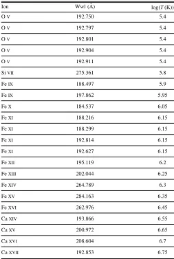
Hinode/EIS Spectral Line List(and their Peak Formation Temperature)used for the VDEM Analysis of EIS Active Region Observations of Figure3
Ion Wwl(Å) log( ( ))T K
OV 192.750 5.4
OV 192.797 5.4
OV 192.801 5.4
OV 192.904 5.4
OV 192.911 5.4
SiVII 275.361 5.8
FeIX 188.497 5.9
FeIX 197.862 5.95
FeX 184.537 6.05
FeXI 188.216 6.15
FeXI 188.299 6.15
FeXI 192.814 6.15
FeXI 192.627 6.15
FeXII 195.119 6.2
FeXIII 202.044 6.25
FeXIV 264.789 6.3
FeXV 284.163 6.35
FeXVI 262.976 6.45
CaXIV 193.866 6.55
CaXV 200.972 6.65
CaXVI 208.604 6.7
spectral decomposition code on the synthetic MUSE data from all three passbands to determine the VDEMS. As mentioned, this inverted VDEMS is not the end goal, but instead can be used to reconstruct the dominant spectral lines without contribution from other nondominant spectral lines and removing the confusion from adjacent slits.
The example in Figure4compares the synthetic FeIX171Å intensity map from the 3D radiative MHD flare simulation
(ground truth, panel (A))with a disambiguated map from the inverted VDEMS(based on synthetic data that includes photon noise, panel(B)). The correlation between the ground truth and intensities derived from the inversions are very good(both for the cases without photon noise, panel (C), and with photon noise, panel (D)), illustrating that the spectral decomposition code accurately disambiguates the MUSE data, even for the challenging scene presented by a flare (in which secondary lines and strong Doppler shifts can potentially lead to multi-slit confusion). Note that this is only shown as an illustration of how the decomposition code can disambiguate multi-slit spectra: in the concept of operations of MUSE, the disambi-guation code would be used to identify locations of multi-slit confusion so that users can isolate signals from secondary lines or a neighboring slit before analyzing the primary lines. For the application of this method to MUSE data, a more detailed description of the various trade-offs and optimal choices for velocity bins, temperature bins, and inversion parameters, as well as the dependence on abundance, density, and noise, will be provided in a follow-up paper (J. Martínez-Sykora et al. 2019, in preparation).
5.3. Slot and Slitless Spectrometers
A special case is when the slit spacingdis equal to the slit width w (in terms of angular coverage over the plane of the sky). This allows us to treat slitless spectrometers and spectrometers with slot modes within this multi-slit framework. An example of a slitless spectrometer is the S082A instrument on Skylab (Tousey et al. 1977). The Coronal Diagnostic Spectrometer on board theSolar and Heliospheric Observatory and the Hinode/EIS instrument (Culhane et al. 2007) are spectrographs with slot modes. The validation of this method to decomposing spectra from these types of instruments like the proposed COronal Spectroscopic Imager in the EUV(COSIE) is detailed in a companion paper(Winebarger et al.2018).
6. Discussion
In this paper, we outlined a general approach to performing the decomposition of spectrograms from astronomical spectrographs with a variety of configurations (e.g., single-slit, multi-slit, and slot mode). The decomposition of spectrograms is not only helpful for removing possible ambiguities(e.g., from which slit this detector signal originated), but such decomposition is also useful for estimating the physical parameters of interest. In this paper and in the companion paper (Winebarger et al. 2018, on decomposing overlappograms from slot spectrometers), we demonstrate application of the technique for interpreting spectro-grams from different instruments observing the solar corona.
[image:7.612.51.565.50.310.2]The applications considered in this paper were for EUV radiation emanating from optically thin plasmas. However, the method is also useful for the interpretation and inversion of
Figure 3.Examples of VDEM inversion applied to actualHinode/EIS active region observations. We considered one of the data sets analyzed by Warren et al.
(2012): AR 11190(centered at[Xcen,Ycen]=[218.1, 304.4]), observed by EIS on 2011 April 15 01:17:19. The top rows show the observed EIS spectral regions used
spectra from optically thick plasmas. Suppose the spectrometer is designed to detect an atomic absorption line formed in the
(partially) optically thick photospheres or chromospheres of astrophysical objects. The emergent spectrum from the optically thick material depends on a number of physical parameters describing the atmosphere including the number density of the absorbing species, the ambient temperature, the slope of the source functionSν(τ)as a function of optical depth
τ, the local magnetic field (if magneto-optical effects like Zeeman splitting are important), and more(especially if the line does not form in local thermodynamic equilibrium). Never-theless, given a physics model including the desired effects, one can construct a library of emergence spectra over parameter space, and fold them through the optical model Oto compute the response matrix R. Seeking a solution along the lines of Equation (6) remains an attempt to express the measured spectrogram as the linear superposition of spectra from the library of atmospheric models. However, since the operatorPis not linear for optically thick radiation, the components of the solution vectorx cannot be interpreted as a density of emitting material (in the case of optically thin EUV radiation, this density is the emission measure)along a single ray. Instead, the linearity should be attributed to the optical characteristics of the instrument (i.e., the operatorO).
Within the framework presented here, a single component inversion is equivalent to seeking to describe the spectrogramy with a single response vector r( )f. Unless one is certain the object is spatially resolved given the telescope PSF, there is perhaps no compelling justification(other than computational
expediency)for a single component inversion. For instance, a spatially extended PSF would lead to the addition of signal associated with photons from different parts of an astrophysical object.
The multi-slit configuration of an instrument like MUSE can be thought of as having a spatially extended (over multiple slits)PSF. But even in the absence of multiple slits, the PSF of a telescope can be sufficiently extended that variations of the physical parameters of interest in the plane of the sky are not resolved. In such cases, the inversion of an observed spectro-gram with a single atmospheric model (i.e., single set of physical parameters) may yield systematic errors. It is then perhaps more appropriate to fit the spectrogram with a linear combination of atmospheric models. Whether such an approach yields superior results over single component inversion remains to be tested and validated. The metrics of interest would depend on the specific use case and are outside the scope of this paper. In this article, we outlined a novel framework for multi-component decomposition of astronomical spectra. We have illustrated application of the method to solar observing instruments, but it can also be used for the interpretation of spectra from other astrophysical sources.
The MUSE team acknowledges support from NASA contract 80GSFC18C0012 to LMSAL. M.C.M.C., B.D.P., J.M.S., and P.T. acknowledge support by NASA’s Heliophy-sics Grand Challenges Research grantPhysics and Diagnostics
of the Drivers of Solar Eruptions(NNX14AI14G to LMSAL).
[image:8.612.64.550.53.343.2]P.A. acknowledges funding from his STFC Ernest Rutherford
Fellowship (grant agreement No. ST/R004285/1). A.D. acknowledges support by NASAs Heliophysics Technology and Instrument Development for Science grant,High Efficiency EUV Gratings for Heliophysics. A.D. acknowledges supportfrom the NASA Heliophysics Technology and InstrumentDevelop-ment for Science award 16-HTIDS16_2-0064, HighEfficiency EUV Gratings for Heliophysics.
ORCID iDs
Mark C. M. Cheung https://orcid.org/ 0000-0003-2110-9753
Bart De Pontieu https://orcid.org/0000-0002-8370-952X Juan Martínez-Sykora https://orcid.org/ 0000-0002-0333-5717
Paola Testa https://orcid.org/0000-0002-0405-0668 Amy R. Winebarger https://orcid.org/ 0000-0002-5608-531X
Adrian Daw https://orcid.org/0000-0002-9288-6210 Viggo Hansteen https://orcid.org/0000-0003-0975-6659 Patrick Antolin https://orcid.org/0000-0003-1529-4681 Theodore D. Tarbell https://orcid.org/ 0000-0002-6294-3026
Peter Young https://orcid.org/0000-0001-9034-2925
References
Boerner, P., Edwards, C., Lemen, J., et al. 2012,SoPh,275, 41 Brooks, D. H., & Warren, H. P. 2016,ApJ,820, 63
Chen, S. S., Donoho, D. L., & Saunders, M. A. 2001,SIAMR,43, 129 Cheung, M. C. M., Boerner, P., Schrijver, C. J., et al. 2015,ApJ,807, 143 Cheung, M. C. M., Rempel, M., Chintzoglou, G., et al. 2019,NatAs,3, 160 Culhane, J. L., Harra, L. K., James, A. M., et al. 2007,SoPh,243, 19 Del Zanna, G. 2008,A&A,481, L49
Del Zanna, G., Dere, K. P., Young, P. R., Landi, E., & Mason, H. E. 2015, A&A,582, A56
Dere, K. P., Landi, E., Mason, H. E., Monsignori Fossi, B. C., & Young, P. R. 1997,A&AS,125, 149
Doschek, G. A., Warren, H. P., & Young, P. R. 2013,ApJ,767, 55 Harra, L. K., Sakao, T., Mandrini, C. H., et al. 2008,ApJL,676, L147 Kosugi, T., Matsuzaki, K., Sakao, T., et al. 2007,Solar Phys.,243, 3 Landi, E., Young, P. R., Dere, K. P., Del Zanna, G., & Mason, H. E. 2013,
ApJ,763, 86
Lemen, J. R., Title, A. M., Akin, D. J., et al. 2012,SoPh,275, 17
Martínez-Sykora, J., De Pontieu, B., Testa, P., & Hansteen, V. 2011,ApJ, 743, 23
Pedregosa, F., Varoquaux, G., Gramfort, A., et al. 2011, JMLR, 12, 2825 Pesnell, W. D., Thompson, B. J., & Chamberlin, P. C. 2012,SoPh,275, 3 Polito, V., Dudík, J., Kašparová, J., et al. 2018,ApJ,864, 63
Tarbell, T. D., & De Pontieu, B. 2017, AAS/Solar Physics Division Meeting, 48, 110.08
Testa, P., De Pontieu, B., Martínez-Sykora, J., Hansteen, V., & Carlsson, M. 2012,ApJ,758, 54
Tibshirani, R. 1996,J. Royal Stat. Soc. B.(Methodological), 58, 267 Tousey, R., Bartoe, J. D. F., Brueckner, G. E., & Purcell, J. D. 1977,ApOpt,
16, 870
van Ballegooijen, A. A., Asgari-Targhi, M., & Voss, A. 2017,ApJ,849, 46 Warren, H. P., Ugarte-Urra, I., Young, P. R., & Stenborg, G. 2011,ApJ,
727, 58
Warren, H. P., Winebarger, A. R., & Brooks, D. H. 2012,ApJ,759, 141 Winebarger, A., Weber, M., Bethge, C., et al. 2018, arXiv:1811.08329 Young, P. R., & Landi, E. 2009,ApJ,707, 173