An Internally Consistent Approach to the Estimation of Market Power and Cost Efficiency with an Application to U S Banking

Munich Personal RePEc Archive

An Internally Consistent Approach to

the Estimation of Market Power and

Cost Efficiency with an Application to

U.S. Banking

Tsionas, Mike and Malikov, Emir and Kumbhakar, Subal C.

Lancaster University Management School, Auburn University, State

University of New York at Binghamton

2018

An Internally Consistent Approach to the Estimation of

Market Power and Cost Efficiency with an Application

to U.S. Banking

∗

Efthymios G. Tsionas1 Emir Malikov2 Subal C. Kumbhakar3,4

1_{Department of Economics, Lancaster University Management School, Lancaster, United Kingdom}

2

Department of Agricultural Economics & Rural Sociology, Auburn University, Auburn, AL, United States 3

Department of Economics, State University of New York at Binghamton, Binghamton, NY, United States 4

University of Stavanger Business School, Stavanger, Norway

April 9, 2018

Abstract

We develop a novel unified econometric methodology for the formal examination of the market power – cost efficiency nexus. Our approach can meaningfully accommodate a mutually de-pendent relationship between the firm’s cost efficiency and marker power (as measured by the Lerner index) by explicitly modeling the simultaneous determination of the two in a system of nonlinear equations consisting of the firm’s cost frontier and the revenue-to-cost ratio equation derived from its stochastic revenue function. Our framework places no a priori restrictions on the sign of the dependence between the firm’s market power and efficiency as well as allows for different hierarchical orderings between the two, enabling us to discriminate between competing quiet life and efficient structure hypotheses. Among other benefits, our approach completely obviates the need for second-stage regressions of the cost efficiency estimates on the constructed market power measures which, while widely prevalent in the literature, suffer from multiple econometric problems as well as lack internal consistency/validity. We showcase our methodol-ogy by applying it to a panel of U.S. commercial banks in 1984–2007 using Bayesian MCMC methods.

Keywords: Productivity & Competitiveness, Efficiency, Market Power, Lerner Index, Banks, Quiet Life Hypothesis

JEL Classification: C11, C30, D24, D40, G21

∗_{Email: [email protected] (Tsionas), [email protected] (Malikov), [email protected]} (Kumb-hakar).

1

Introduction

Owing to its important social welfare implications, researchers have long been interested in disen-tangling the complex relationship between the market structure and the cost efficiency of firms. The two notable (structural) hypotheses put forth to conceptualize this relationship — the quiet life and the efficient structure hypotheses (thereafter, QLH and ESH) — contrast rather sharply both in the sign and implied directionality of the relationship. Not only is it still unclear if the relationship is positive or negative, but it also remains unsettled whether the market structure de-termines the firms’ performance, including their efficiency, or whether the market structure should rather be viewed as an endogenous outcome of firms’ behavior reflective (at least partly) of their efficiency levels.

The QLH as postulated by Hicks (1935) conceptualizes the market structure as a determinant of firms’ efficiency, whereby firms with higher market power trade potential monopoly rents for lower efficiency. This negative relationship may exist because, owing to the high levels of market power providing them with the “price cushion”, firm managers might not work as hard to keep costs at minimum or might expend resources to obtain/maintain the market power, i.e., engage in further rent-seeking (Berger & Hannan, 1998). In contrast, Demsetz’s (1973) ESH asserts that the industry market structure is instead an outcome of the interaction among individual firms exhibiting different efficiency levels, through which more efficient firms gain larger market shares and hence secure greater monopolistic power. Such a positive relationship between the cost efficiency and market power is oftentimes rationalized as the result of more efficient firms with superior management out-competing their less efficient rivals which operate at higher costs (Berger, 1995).

Empirical work on the nexus between firm efficiency and market power has particularly favored the U.S. banking sector as a “laboratory” for analysis owing to the relative homogeneity of banks in the industry which helps facilitate cross-firm performance comparisons (e.g., Berger & Hannan, 1998; Jayaratne & Strahan, 1998; Koetter, Kolari & Spierdijk, 2012). The findings, however, have been rather mixed. While Berger & Hannan (1998) and Delis & Tsionas (2009) find that, consistent with the QLH, U.S. banks exhibiting greater market power tend to suffer from significant cost efficiency losses, the finding of a positive relationship between cost efficiency and market power of European banks documented by Weill (2004), Casu & Girardone (2006) and Maudos & Fern´andez de Guevara (2007) instead buttress the ESH. More recently, Koetter et al. (2012) have also reported the empirical evidence pointing to a positive effect of the market power on the bank’s cost efficiency in the U.S. which lends support to ESH.1 _{To the contrary, in line with QLH, Koetter & Vins (2008)}

consistently find a negative relationship between bank-level measures of market power and cost efficiency for German savings banks. Similar findings are reported by Turk Ariss (2010) and Dong, Firth, Hou & Yang (2016) for banks in developing countries including China.

While different in their choice of the measure of market power and in some other methodolog-ical aspects, overwhelming majority of such studies resort to a two-stage analysis which suffers from multiple fundamental econometric problems (discussed below) casting a serious shadow on the validity and reliability of their findings. The same concerns also apply to a broader literature examining the links between the market structure/competition and firms’ profitability, profit ef-ficiency or stability,2 _{which the papers on the cost efficiency – market power nexus closely relate}

1

They do document an opposite finding in support of the QLH using measures ofprofit efficiency. Restrepo-Tob´on & Kumbhakar (2014) however cast doubt on the latter finding in their re-examination of Koetter et al. (2012). 2

to and share much of their methodology with. In this paper, we contribute to the literature by proposing a novel unified econometric approach that tackles the problems associated with such two-stage analyses widely favored in the literature.

To make matters more concrete, we focus on the estimation issues concerning the examination of thefirm-level relationship between the market power and cost efficiency. Thus, we measure firms’ market power using the Lerner index which is a popular go-to firm-specific measure of monopolistic power in the literature (e.g., de Guevara & Maudos, 2007; Berger, Klapper & Turk-Ariss, 2009; Koetter et al., 2012; Das & Kumbhakar, 2016) since the alternative indices such as Herfindahl-type concentration ratios or the Rosse-Panzar H-statistic usually yield industry-level estimates3 of competitiveness in the market (for more on these measures, e.g., see Bolt & Humphrey, 2015). The cost efficiency estimates are obtained using a widely popular stochastic frontier formulation of the cost function (e.g., Berger & Mester, 1997, 2003; Malikov, Kumbhakar & Tsionas, 2016). Traditionally, researchers perform their analyses in two stages, where they first compute the Lerner index using the fitted scale elasticity of cost as well as estimate firm-specific cost efficiency scores and then regress the obtained cost efficiency estimates on the Lerner index in the second stage (e.g., see Maudos & Fern´andez de Guevara, 2007; Koetter & Vins, 2008; Turk Ariss, 2010; Koetter et al., 2012). However, not only does the latter two-stage model lack internal consistency (validity) but it also suffers from a number of acute econometric issues.

Specifically, the two-stage analysis fails to accommodate a simultaneous determination of the Lerner index (firm’s market power) and the cost efficiency. As discussed earlier, the directionality of the relationship between the market power and efficiency is ambiguous, and causality likely runs both ways, whereby more efficient firms are able to survive the competition and thus acquire greater market power which in turn may create “quiet life” incentives leading to a decline in firms’ efficiency. Even if this “reverse causality” problem is acknowledged by researchers, the methodology used to tackle it however usually falls short of its overreaching task. The endogeneity is oftentimes argued to be resolved either by merely “adjusting” the Lerner index whereby the efficiency-corrected estimates of the marginal cost are used in the computation of the index (e.g., Turk Ariss, 2010) and/or by employing instruments in the second-stage regressions of the efficiency estimates on the market power index (e.g., Berger & Hannan, 1998; Berger et al., 2009; Koetter et al., 2012). However, neither of these methods can meaningfully accommodate the simultaneity of the firm’s market power and efficiency. While the “adjusted” Lerner index indeed explicitly acknowledges the existence of cost inefficiency, in its construction however, researchers use the marginal cost estimates from the stochastic cost frontier model that assumes complete independence of the cost (in)efficiency from the cost function covariates and hence the Lerner index. That is, the efficiency-adjusted Lerner index is “adjusted” under the assumption that cost efficiency isindependent from the firm’s market power. Not only may the cost (in)efficiency be severely biased because one forcefully imposes its independence from the market power during the estimation (Delis & Tsionas, 2009), but this independence also suggests that any second-stage regressions of the cost efficiency on the market power indicators (and possibly other contextual variables) contradict the underlying assumption of the first-stage regression and thus are likely to be spurious. Worse yet, the cost inefficiency is oftentimes assumed to be not only independently but also identically distributed across firms with constant mean and variance (e.g., Maudos & Fern´andez de Guevara, 2007; Turk Ariss, 2010; Koetter et al., 2012), which implies no systemic relationship between the firm’s efficiency and other covariates thus rendering any second-stage analysis void. Subsequently, the two-stage methodology lacks internal consistency (validity) by which both stages would be reconcilable with one another.

3

In its second stage, virtually no study recognizes that both the firm’s efficiency and the Lerner index are in fact generated estimates subject to parameter uncertainty which needs to be accounted for when performing inference. While the sampling uncertainty associated with the first-stage estimate used as a left-hand-side variable in the second-stage analysis (usually, cost efficiency) does not generally pose a problem, the same cannot be said about the generated regressor (usually, the Lerner index) used as a right-hand-side explanatory variable. Further, the standard approach, whereby the Lerner index is constructed using raw information on the firm’s revenues and estimates of the marginal cost from a stochastic cost frontier, implicitly assumes away any stochasticity in the firm’s revenue function. The latter is rather arbitrary; it only appears logical to allow for stochastic noise in both the firm’s costs and revenues. Lastly but not least importantly, the second-stage regressions of the cost efficiency scores on the Lerner index are usually estimated via least squares (ordinary or two-stage) without taking a bounded codomain of the cost efficiency estimates (or the log thereof) into consideration (e.g., Berger & Hannan, 1998; Weill, 2004; Koetter et al., 2012).4

In this paper, we seek to offer a solution to the above econometric problems associated with the formal examination of the cost efficiency – market power nexus. More specifically, we propose a novel, internally consistent approach to modeling a mutually dependent relationship between the firm’s cost efficiency and marker power (as measured by the Lerner index), which explicitly accommodates the simultaneous/endogenous determination of the two and completely obviates the need for a second-stage analysis. Both the firm’s cost efficiency and marker power index are estimated jointly and derived from a single unified model thus enabling us to interpret and analyze them on a common ground.

We begin by recognizing that neither the cost efficiency nor the market power are observed and, therefore, ought to be treated accordingly when estimating the firm’s production process. We let both of these latent variables directly co-depend in a variety of ways, thereby having efficiency be automatically adjusted for market power and vice versa, in a system of nonlinear equations consisting of the firm’s cost frontier and the revenue-to-cost ratio equation derived from the firm’s stochastic revenue function. Our framework places no a priori restrictions on the sign of the dependence between market power and efficiency as well as allows for different hierarchical orderings between the two, enabling us to meaningfully discriminate between the QLH and ESH. To draw statistical inference, we consider three alternative econometric specifications of our unified system-based model which we estimate using Markov Chain Monte Carlo (MCMC) methods.

We showcase our unified model by applying it to a panel of U.S. commercial banks operating in 1984–2007. Regardless of the econometric specification of the model used, the data consistently point to a negative dependence between the bank’s cost efficiency and the Lerner index thus provid-ing empirical evidence in support of the QLH. This findprovid-ing is reversed when we employ a traditional two-stage analysis where both the cost efficiency and the adjusted Lerner index are estimated sep-arately without allowing for a simultaneous determination of the two. The latter highlights the pivotal importance of a proper econometric modeling of the market power – efficiency relationship which a popular two-stage analysis is unable to deliver.

The rest of the paper proceeds as follows. Section 2 introduces our unified model of market power and efficiency. We describe three alternative econometric specifications of our model in Section 3 with the details relegated to the Appendix. Section 4 reports the empirical application. We conclude in Section 5.

4

2

A Unified Model

In this section, we propose a novel, internally consistent approach to modeling a mutually dependent relationship between the firm’s cost efficiency and marker power (as measured by the Lerner index), which explicitly accommodates the simultaneous/endogenous determination of the two.

For the ease of exposition, we first consider the case where a firm, which may potentially exercise monopoly power in the market, produces asingle output. Suppose the firm’s cost function is given by C = C(w, y) _≡ minx {w′x|y≤F(x)} : RJ++×R+ → R+, where x ∈ RJ+ is the vector of

inputs with the corresponding vector of input prices w_∈RJ_{++,y is the total output quantity, and}

F(x) is the production function. Further, let the output price be denoted byp_∈R_{++. To measure}

the firm’s market power, we use the Lerner index widely favored in the literature. Specifically, we define the Lerner index of market power as follows: Le = p₋ ∂C(w,y)

∂y

/p _∈ [0,1), where ∂C(w,y) ∂y

is the firm’s marginal cost. The rationale of the index is that the monopolistic firm can set the price above the marginal cost (which normally equals the competitive price) and, therefore, the excess of price over marginal cost should be a good measure of market power. Higher values of the index imply greater market power, whereas the zero value (a lower boundary) points to a perfectly competitive firm. Lastly, note that the Lerner index is closely related to the conventional measure of the firm’s markup which uses the marginal cost, as opposed to the output price, as the reference for sizing the firm’s monopoly power, namely p₋∂C(w,y)

∂y

∂C(w,y) ∂y .

We next rewrite the Lerner indexLeas a function of the firm’s revenue and the output elasticity of its cost. Specifically,

e

L= p−

∂C(w,y) ∂y

p =

p₋ C_{y ×}εy

p =

R₋C_×εy

R , (2.1)

whereεy = ∂ln_∂C_ln(w_y,y) is the output (scale) elasticity of cost, andR=py∈R+is the total revenue.

From (2.1), it is immediately evident that, had the output elasticity of cost εy been known

and/or directly observable from the data, we could have easily obtained the estimate of the Lerner index. However, given the unobservability ofεy, we need to estimate it too. To do so, we can make

use of the information from the firm’s cost function.5

Before proceeding to the details of how the output elasticity of cost is estimated, we first generalize the above discussion to the case when the firm engages in a multi-output production. The firm’s multi-output cost function can then be redefined as

C =C(w,y)_≡min

x

w′x_|T(x,y)_≥1 :RJ_++×RM_{+ →}R₊, (2.2)

where y _∈ RM_{+ is the vector of outputs, T(·) is the transformation function relating inputs to}

outputs within the set of technologically feasible combinationsT_{={(x,y) :x can producey}, and} xand w are just as defined earlier. The vector of output prices is now given byp_∈RM_++.

In the instance of M outputs being produced by the firm, it is now imperative to recognize that, following our earlier definition, one can defineM different output-specific Lerner indices, i.e.,

e

Lm = pm − ∂C_∂y(w_m,y)/pm ∀ m = 1, . . . , M, with the corresponding M output-specific markup

measures. To get around this issue, we therefore employ a multi-output definition of the Lerner index where the market power is gauged on the basis of the differential between the firm’s average total revenue (as opposed to the price) and its “average” marginal cost (e.g., Koetter & Poghosyan,

5

2009; Koetter et al., 2012; Das & Kumbhakar, 2016). Similar to (2.1), the multi-output Lerner index can then be written as

L= R−C×

P mεym

R , (2.3)

whereεym =

∂lnC(w,y)

∂lnym is the elasticity of cost with respect to themth output, andR=

P

mpmym∈

R_{+is the total revenue as defined earlier. Essentially, such an index provides a measure of the firm’s}

“average” monopolistic power across the output markets. From (2.3), it follows that

R C =

1 1₋L×

X

m

εym, (2.4)

which in logs yields

ln

R C

= ln X

m

εym

!

+uL, (2.5)

where, given the permissible range of the Lerner index, we define the (latent) unbounded one-sided transformation ofL asuL=−ln(1−L)≥0 which is increasing in the firm’s marker power.

Since the so-called “scale elasticity” P_mεym is unobservable for a direct computation of uL

(and hence ofL), we recover it from the firm’s dual cost function which we estimate simultaneously along with equation (2.5) while also allowing for(i) the presence of one-sided cost inefficiency and (ii) mutual dependence between the latter and the Lerner index. Formally, after appending both equations with two-sided stochastic errors, the nonlinear system of simultaneous equations, which we seek to estimate, is given by

lnC= ln_C(w,y;β) +uC+vC (2.6a)

ln

R C

= ln X

m

εym(w,y;β)

!

+uL+vL, (2.6b)

where ln_C(_· ;β) is some parametric specification of the unknown cost function with β being the vector of unknown parameters, and uC ≥ 0 is the one-sided cost inefficiency term. Here, we

explicitly recognize thatεym is a function of the unknown parametersβ, since the output elasticity

of cost is found as the partial log-derivative of the fitted cost function, i.e.,εym=

∂lnC(w,y;β)

∂lnym ∀m=

1, . . . , M. Following the popular practice, we use the translog specification for ln_C(_·;β), known to yield a flexible second-order approximation to an arbitrary, unknown functional form for the cost function.

Our system-of-equations approach presents a superior alternative to the standard practice of empirical assessment of the efficiency – market power relationship in the literature, whereby one first estimates the firm’s cost function to obtain estimates of cost efficiency and scale elasticity and then, as a second step, uses the latter to compute the Lerner index. Having done the above, a common researcher then proceeds to the second-stage regressions of the efficiency estimates on the Lerner index estimates and, potentially, some other covariates. In principle, there are multiple problematic issues with this practice (as discussed in detail in Introduction) including the lack of internal consistency/validity. Therefore, to ensure the coherence and internal consistency of the econometric model used for the analysis of the market power – cost efficiency relationship, it is pivotal that one estimates the firm’s level of efficiency and market power jointly while allowing for potential dependence not only between stochastic noises vC and vL, owing to the

seemingly-unrelated-regressions structure of model in (2.6), but also betweenuC anduLthemselves. Not only

the need for a second-stage analysis plundered by numerous econometric problems. In fact, explicit modeling of the potential dependence betweenuC anduLis the key to a consistent6 testing of the

QLH versus ESH. Unfortunately, statistical inference in this context is quite complicated due to the fact that both the cost inefficiency and the market power are unobserved latent variables which are one-sided and correlated. Thus, formal statistical discrimination between the QLH and ESH may be a rather burdensome task.

3

Econometric Specification

Our model of endogenous (simultaneous) interplay between the firm’s cost efficiency and market power in (2.6) can be formalized econometrically in the number of ways. In what follow, we propose three alternative methods of modeling the market power – cost efficiency relationship, which differ in their formulation of the cross-equation dependence between (2.6a) and (2.6b). Regardless of the specifics, all three models accommodate mutual dependence of the cost inefficiencyuC and the

log-Lerner-index function uL via a simultaneous-equations structure.

In Model I, we take the most “agnostic” view of directionality of the relationship between the firm’s cost efficiency and market power by imposing no structure onto the order of causality in their interdependence. We do so by modeling their joint one-sided distribution with the dependence being controlled by the covariance parameter. As an alternative, Model II postulates an a priori hierarchical dependence between cost efficiency and market power, whereby the latter is permitted to directly affect the latent inefficiency term via its mean. Model III relaxes Model II by explicitly allowing for bidirectional cross-equation effects between cost efficiency and market power working through their respective means. Thus, in contrast to Model I which also accommodates bidirectional effects but does so via a single dependence parameter, Model III allows one to directly examine if both directions are significant (owing to the model’s explicit two-parameter formulation of the cross-equation dependence). However, neither of the three model specifications impose restrictions onto signs of the parameters controlling the dependence between uC and uL. Ultimately, the data

are to tell which model describes them more adequately.

To aid the discussion, we first rewrite our system of equations in (2.6) in a stylized form:

y1,it =x′itβ+v1,it+u1,it (3.1a)

y2,it =f(xit;β) +v2,it+u2,it ∀ i= 1, . . . , n; t= 1, . . . , T, (3.1b)

where y1,it and xit denote lnCit and the associated translog expansion of the cost determinants,

respectively; y2,it denotes ln(Rit/Cit);f(xit;β)≡ln (P_mεym) denotes the log of scale elasticity of

cost defined as the sum of output elasticities derived by differentiating the translog cost function specification with respect to the log outputs; and β is a k_×1 vector of unknown parameters to be estimated. (The details of the MCMC techniques used to estimate each of the three models are relegated to the Appendix.)

3.1 Model I: Dependence via Joint Distribution

In Model I, the cost inefficiency u1 and the log-Lerner-index function u2 are postulated to be

mutually dependent by following a joint one-sided distribution with the dependence between the two being controlled by the covariance parameter. Formally, the stochastic assumptions for Model

6

I are as follows:

v1,it

v2,it

∼ N_{(0,Σ), (3.2a)}

u1,it

u2,it

∼ N+₍µ,Ω), u1,it ≥0, u2,it ≥0, (3.2b)

independently of each other as well as of the regressorsxit, whereµ= [µ1, µ2]′andΩ=

ω11 ω12

ω12 ω22

. For the ease of exposition, in the remainder of this subsection, we treat (µ1, µ2) as constants.

However, we can easily allow the means ofu1,itandu2,itto vary with some contextual covariates via

the following parameterization: µ1,it =z′1,itγ1 and µ2,it =z′2,itγ2, wherez1,it and z2,it is anl1×1

and l2×1 vector of covariates, andγ1 and γ2 is an l1×1 and l2×1 vector of the corresponding

parameters, respectively. In fact, we do so in the empirical application, where we let µ1 and µ2 be

time-varying and firm-specific by conditioning them on heterogeneous firm characteristics.

Next, we writexit=x′_o,it,x_∗′_,it′, wherexo,itis ako×1 vector corresponding to the linear terms

in the translog expansion. The scale elasticity P_mεym,it can then be computed as

P

mεym,it = x′_o,itRβ, whereRis ako×kselection matrix whose elements are either 0 or 1. Also, for convenience,

defineyit= [y1,it, y2,it]′,vit= [v1,it, v2,it]′ and uit= [u1,it, u2,it]′.

The conditional distribution of the observables is given by

p(yit|xit,θ) = (2π)−1CΩ|Σ|−1/2×

Z _∞

0

Z _∞

0

exp

−1₂(rit−uit)′Σ−1(rit−uit)−

1

2(uit−µ)

′_Ω−1_(u

it−µ)

duit,

(3.3)

whererit =yit−

x′_itβ

f(xit;β)

,CΩ = (2π)−1|Ω|−1/2Φρ

µ1 ω11,

µ2 ω22

−1

is the normalizing constant of the bivariate truncated normal distribution with Φρdenoting the bivariate standard normal distribution

function with the correlation coefficientρ=ω12(ω11ω22)−1/2, andθ=β′, vech(Σ)′, vech(Ω)′,µ′′

denotes the collective vector of all parameters.

It is straightforward but tedious to generalize Pitt & Lee (1981, Appendix 2) and express (3.3) in the following form:

p(yit|xit,θ)∝ |Ω|−1/2|Σ|−1/2Φρ

Ω−_diag1 µ−1Φρ

V−_diag1 µ∗_itexp

−1₂Qit

, (3.4)

where V−1 = Σ−1 +Ω−1, µ∗_it = V Ω−1µ+Σ−1rit, Qit = (rit−r∗it)W−1(rit−r∗it) +µ′Aµ

such that W−1 = Σ−1 ₋Σ−1VΣ−1, A = Ω−1 ₋Ω−1 V+VΣ−1WΣ−1VΩ−1 and r∗_it =

WΣ−1VΩ−1µ. Lastly, Mdiag denotes the diagonal matrix which contains main diagonal elements

of some matrix M.

To obtain (3.4), let _X = (rit−uit)′Σ−1(rit−uit) + 1₂(ui−µ)′Ω−1(uit−µ) so that the

in-tegral in (3.3) becomes _I = R_Rd

−

exp₋1_2X du with d = 2, and it is more convenient to work with the convolution r = v+u when u _∈ Rd_{− (i.e.,} uit ≤ 0). Completing the square, we

ob-tain _X = _Xo+C, where Xo = (u−µ∗)′V−1(u−µ∗) and C = r′Σ−1r+µ′Ω−1µ−µ∗′V−1µ∗.

The latter term, which does not depend on u, can be factorized (like we have shown above) as

C = (r₋r∗)W−1(r₋r∗) +µ′Aµ. Thus, dealing with _I requires that we compute the inte-gral _Io = R_Rd

−

exp₋1_2Xo du by converting it to the integral of the multivariate standard

zi = (ui−µ∗i)/

√

Vii ∀ i = 1, . . . , d and ρV is the correlation matrix corresponding to the

covari-ance matrix V whose main diagonal elements are denoted by Vii. Then, it is straightforward to

show that _Io =R_Rd

−

exp₋1_2Xo du = 2πQdi=1Vii 1/2

|ρ_V|1/2ΦρV

· · ·,₋µ∗

iV−

1/2

ii ,· · ·

, or Io =

2π_|V_|1/2ΦρV

· · · ,₋µ∗

iV−

1/2

ii ,· · ·

, where ΦρV(b) = (2π)

−d/2_|ρ

V|−1/2 R_Q

d

i=1(−∞,bi]exp

−12z′ρ−V1z dz.

Here, we generalize Pitt & Lee’s (1981) results in two important ways. First, we allow for a general matrix Σ. Second, we allow for a multivariate truncated normal distribution of uit.

With the convention that Φρ denotes thed-variate standard normal distribution function with the

correlation matrixρ=hωij(ωiiωjj)−1/2; i, j= 1, . . . , d i

, the formula in (3.4) applies to the general

d-dimensional multivariate case.

3.2 Model II: Hierarchical Dependence

In contrast to Model I which imposes no structure onto the order of causality in the dependence between cost efficiency and market power, Model II postulates ana priori hierarchical dependence betweenu1,itandu2,it, whereby the former follows a one-sided distribution conditional on the latent

market power which, in turn, also follows a one-sided distribution. More specifically, we make the following stochastic assumptions for Model II:

v1,it

v2,it

∼ N_{(0,Σ), (3.5a)}

u1,it|u2,it ∼ N+ z1′,itγ1+ψ1u2,it, ω12

, (3.5b)

u2,it ∼ N+ z′2,itγ2, ω22

. (3.5c)

In this model, the latent market power is dependent on a vector of contextual covariatesz2,it and

follows a truncated normal distribution to ensure its non-negativity. The latent cost inefficiency, which depends on a vector of contextual covariates z1,it, follows a truncated normal distribution

and, importantly, is also affected by the latent market power through its mean.

We note that the specification of the hierarchical dependence between u1,it andu2,it in (3.5) is

different from that implied by the bivariate truncated normal distribution employed in Model I. To see this clearly, recognize that, if uit ∼ N+(z′1,itγ1)′,(z′2,itγ2)′

′_{,Ω, then it follows that}

u1,it|u2,it ∼ N+

z′_1,itγ₁+ω12

ω22

u2,it−z′2,itγ2

, ω11−

ω₁₂2 ω22

(3.6a)

u2,it|u1,it ∼ N+

z′_2,itγ₂+ω12

ω11

u1,it−z′1,itγ1

, ω22−

ω2 12

ω11

, (3.6b)

implying that the two variables are dependent through the covariance parameter ω12. Therefore,

the hierarchical dependence is different from the dependence implied by the joint specification.

3.3 Model III: Dependence via Conditional Distributions

Model III relaxes Model II further by also allowing for the dependence of the latent market power on the cost efficiency via its own conditional distribution. Thus, the cross-equation dependence is now explicitly bidirectional. That is, we assume that

v1,it

v2,it

u1,it|u2,it ∼ N+ z1′,itγ1+ψ1u2,it, ω12

, (3.7b)

u2,it|u1,it ∼ N+ z2′,itγ2+ψ2u1,it, ω22

. (3.7c)

Clearly, this model (like the previous two) does not a priori restrict signs of the parameters controlling the dependence between u1 and u2 in the two conditional distributions:

p(u1,it|u2,it,·) = 2πω21

−1/2

exp

− 1

2ω2 1

u1,it−z′1,itγ1−ψ1u2,it2

×

Φ z′_1,itγ₁+ψ1u2,it/ω1−1✶(u1,it≥0) (3.8)

and

p(u2,it|u1,it,·) = 2πω22

−1/2

exp

− 1

2ω₂2 ui2−z

′

2,itγ2−ψ2u1,it2

×

Φ z′_2,itγ₂+ψ2u1,it/ω2−1✶(u2,it≥0). (3.9)

The joint distribution p(u1,it, u2,it|·) =p(u1,it|u2,it,·)p(u2,it|·) = p(u2,it|u1,it,·)p(u1,it|·) is

un-available given that the marginal distributions are not specified. Combining with the relevant terms in the posterior kernel distribution, we have

p(u1,it, u2,it|Ξ,θ) = exp

−1₂(uit−rit)′Σ−1(uit−rit)

p(u1,it, u2,it|·), (3.10)

whereΞdenotes the available data.

4

Empirical Application

We showcase our proposed unified system-based model by applying it to study the interplay between monopolistic power and cost efficiency in the U.S. commercial banking industry.

4.1 Data

The annual bank-level year-end data that we use in this paper come from Koetter et al. (2012) and originate in Call Reports of the Federal Reserve System. The sample includes all FDIC-insured commercial banks with available data between 1984 and 2007. We exclude banks reporting negative values for assets, equity, outputs and prices. Following Stiroh & Strahan (2003) and Koetter et al. (2012), we also exclude banks in the District of Columbia and South Dakota due to their exceptional laws concerning the credit card business practices. To mitigate the influence of outliers, we also truncate input prices at the 1st and 99th percentiles of their respective empirical distributions. All nominal quantities are deflated using the 2005 Consumer Price Index for all urban consumption published by the U.S. Bureau of Labor Statistics. The operational dataset is an unbalanced panel of 17,148 banks with a total of 216,737 observations.

We model the bank’s production technology using the commonly used “intermediation ap-proach” of Sealey & Lindley (1977), according to which a bank’s balance sheet is assumed to capture the essential structure of its core business. Liabilities, together with physical capital and labor, are taken as inputs to the bank’s production process, whereas assets (other than physical) are considered as outputs. Specifically, we define two output variables: securities (y1) and loans

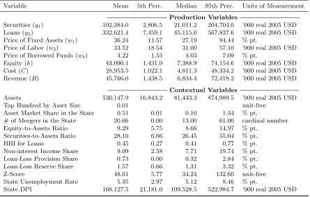
Table 1. Data Summary Statistics

Variable Mean 5th Perc. Median 95th Perc. Units of Measurement Production Variables

Securities (y1) 102,384.0 2,806.5 21,011.2 204,704.0 ’000 real 2005 USD Loans (y2) 332,621.4 7,459.1 45,115.0 567,837.6 ’000 real 2005 USD Price of Fixed Assets (w1) 36.24 11.57 27.19 94.44 % pt.

Price of Labor (w2) 33.52 18.54 31.00 57.10 ’000 real 2005 USD Price of Borrowed Funds (w3) 4.22 1.55 4.03 7.09 % pt.

Equity (k) 43,090.1 1,431.0 7,388.9 74,154.6 ’000 real 2005 USD Cost (C) 28,953.5 1,022.1 4,811.3 48,334.2 ’000 real 2005 USD Revenue (R) 45,766.0 1,438.5 6,834.4 72,418.2 ’000 real 2005 USD

Contextual Variables

Assets 530,147.9 16,843.2 81,443.3 874,989.5 ’000 real 2005 USD Top Hundred by Asset Size 0.01 unit-free

Asset Market Share in the State 0.51 0.01 0.10 1.34 % pt.

# of Mergers in the State 20.66 0.00 13.00 61.00 cardinal number Equity-to-Assets Ratio 9.29 5.75 8.66 14.97 % pt.

Securities-to-Assets Ratio 28.10 6.66 26.45 55.04 % pt. HHI for Loans 0.45 0.27 0.41 0.77 % pt. Non-interest Income Share 9.09 2.58 7.71 19.74 % pt. Loan-Loss Provision Share 0.73 0.00 0.32 2.84 % pt. Loan-Loss Reserve Share 1.57 0.66 1.31 3.32 % pt. Z-Score 48.01 5.77 34.24 132.60 unit-free State Unemployment Rate 5.35 2.97 5.12 8.46 % pt.

State DPI 168,127.5 21,181.0 109,528.5 522,984.7 ’000 real 2005 USD

the sum of expenses on these inputs. Input prices (w1, w2, w3) are obtained by dividing expenses

on these items by their respective quantities. We also include equity capital (k) as an additional input to the production technology. The treatment of equity as an input to banking production technology is usually motivated by the argument that banks may use the latter as a source of loanable funds and thus as a cushion against losses. Due to the unavailability of the price of equity, we follow Berger & Mester (1997, 2003) in modelingk as a quasi-fixed input. Total revenue (R) is the sum of revenues from the two output categories.

Table 2. Posterior Mean Estimates of Scale Elasticity

Model Mean Estimate 95% Bayes Interval (I) 0.8677 (0.8014; 0.9336) (II) 0.9083 (0.8147; 1.0010) (III) 0.8359 (0.7581; 0.9136) (IV) 0.8858 (0.8220; 0.9496)

market; (v) the bank’s ratio of equity to total assets measuring its capitalization is meant to control for factors contributing to bank distress (e.g., Gan, 2004); (vi) the bank’s ratio of securities to total assets, (vii) the Hirschman-Herfindahl index across the banks’ different types of loans and (viii) the share of non-interest income are all controlling for the possibility that greater competition might entice banks to engage in nontraditional activities as well as to more actively seek diversification of their portfolio (Koetter et al., 2012); (ix) the share of loan-loss provisions and (x) loan-loss reserves in the bank’s total loans proxy for the credit risk, whereas (xi) the bank’s z-score7 proxies for the overall risk of bank failure; (xii) the disposable personal income and (xiii) the unemployment rate in the state are the controls for macroeconomic conditions which may affect the competition (Chirinko & Fazzari, 2000) as well as efficiency. We also include three indicator variables reflective of institu-tional changes in states that correspond to deregulation in the intrastate branching (by means of mergers and acquisitions), the interstate expansion (via bistate agreements) and the post-IBBEA interstate banking. The chosen contextual variables are all likely to greatly influence bank’s busi-ness strategies in pursuit of the maximum franchise value (Demsetz, Saidenberg & Strahan, 1996; DeYoung & Rice, 2004) with important implications for its efficiency and/or market power. See Table 1 of Koetter et al. (2012) for details on the construction and rationale behind the variables. Table 1 above presents the data summary statistics.

4.2 Results

In this section, we report the results from our unified system-based model in (2.6) estimated using the three specifications described in Section 3. These econometric models are respectively referred to as the Model I, II and III. In all three cases, we assume the translog cost function and allow for non-neutral temporal shifts in the bank’s cost frontier as well as let the means of latentuC anduL

be time-varying and bank-specific conditional on the contextual variables capturing heterogeneous bank characteristics. In line with the intuition outlined earlier, we include the contextual variables summarized in Section 4.1 in the covariate set of the mean function of cost inefficiencyuC and/or

the log-Lerner-index function uL; both means also include the time trend and its square. (For

complete variable lists corresponding to each mean function, see Table 4). The bank’s cost efficiency is computed as exp_{−buC}, whereas the (automatically adjusted) Lerner index is recovered as 1−

exp_{−u_bL}.

To highlight the merits of our proposed system-based approach, we also examine the relationship between market power and cost efficiency employing the most popular strategy in the literature whereby we estimate the stochastic cost frontier in (2.6a) alone without accounting for the joint dependence of the Lerner index and efficiency. Following Koetter et al. (2012) and many others, the fitted cost frontier is then used along with raw data on total revenues to construct the “adjusted” Lerner index as follows: Lb = R₋Cb_×P_mε_bym

/R, where both Cb and ε_bym are obtained from

the estimated stochastic cost frontier. The relation between the cost efficiency estimates and the

7

Table 3. Posterior Mean Estimates of Cost Efficiency and Market Power

Model Mean Estimate 95% Bayes Interval Model I

Efficiency 0.8230 (0.7928; 0.8534) Lerner Index 0.3349 (0.2885; 0.3812)

Model II

Efficiency 0.8090 (0.7530; 0.8649) Lerner Index 0.3321 (0.2737; 0.3904)

Model III

Efficiency 0.7983 (0.7288; 0.8675) Lerner Index 0.3589 (0.3015; 0.4165)

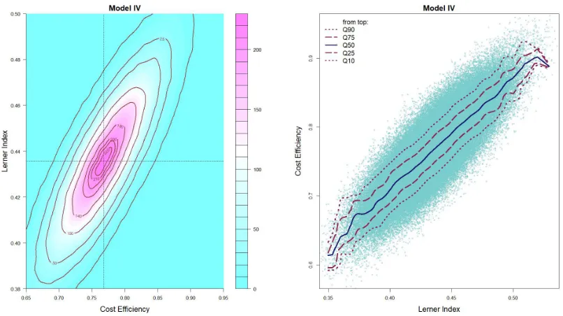
Model IV

Efficiency 0.7675 (0.6704; 0.8644) Lerner Index 0.4356 (0.3858; 0.4854)

Lerner index is then analyzed in the second stage. We refer to this model hereinafter as Model IV. It is primarily meant to illustrate the empirical sensitivity of the findings to proper modeling of the simultaneous determination of both the bank’s efficiency and market power.

Before we proceed to the discussion of the main results concerning the market power – efficiency nexus and its accompanying hypotheses, we first examine the estimates of the scale elasticity. The posterior mean estimates ofεyalong with their 95% credible interval from the four estimated models

are reported in Table 2. The estimates are of interest because they gauge returns to scale in the industry. Specifically, the bank is said to exhibit increasing/constant/decreasing returns to scale if the scale elasticity (of cost) is less than/equal to/greater than one. While the posterior mean (point) estimates from all four models suggest that, on average, banks operate at increasing returns to scale during our sample period, in the case of Model II the 95% posterior coverage region includes unity thereby suggesting roughly constant returns to scale. All other models however indicate that the banking industry exhibits significant scale economies, consistent with the recent findings (e.g., Wheelock & Wilson, 2012; Hughes & Mester, 2013; Malikov, Restrepo-Tob´on & Kumbhakar, 2015). Table 3 presents the estimates of primary interest to our paper. The reported are the posterior mean estimates of the bank’s cost efficiency and the Lerner index from the four models over the entire sample. Among the three specifications of our system-based approach, Model I yields the highest estimates of the mean cost efficiency for banks at around 0.82, while Model III produces the lowest estimates that are, on average, about 2.5 basis points lower. Interestingly, when we estimate the cost frontier without any accommodation of the joint dependence of the bank’s market power and efficiency (Model IV), we obtain efficiency scores that are even lower with the average posterior estimate of 0.77. The differences in results from the two types of models (our preferred system-based estimator vs. a more popular single-equation specification) are more evident when we contrast their estimates of the Lerner index. Model IV appears to over-estimate the monopolistic power exercised by the banks in our sample, with the pooled mean posterior estimate being as high as 0.44 versus the value of the corresponding statistic from our system-based Models I–III ranging between 0.33 and 0.36.

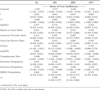
Table 4. Posterior Mean Estimates of Parameters across Models I–IV

(I) (II) (III) (IV)

Mean of Cost Inefficiency

Constant –1.335 –0.717 –0.445 –0.373 (–1.515; –0.877) (–0.944; –0.342) (–0.525; –0.316) (–0.551; –0.212) t 0.035 0.042 0.017 0.005

(0.017; 0.044) (0.030; 0.052) (0.012; 0.023) (0.002; 0.013) t2

–0.004 0.003 0.001 0.001 (–0.006; –0.002) (–0.004; 0.005) (–0.002; 0.003) (–0.002; 0.003) log(Size) 0.377 0.173 0.216 0.105

(0.221; 0.414) (0.005; 0.224) (0.130; 0.245) (0.007; 0.155) Equity-to-Assets Ratio 0.251 0.180 0.313 0.216

(0.181; 0.322) (0.103; 0.199) (0.277; 0.366) (0.189; 0.256) Loan-Loss Provision Share 0.414 0.255 0.202 0.104

(0.303; 0.525) (0.188; 0.344) (0.177; 0.287) (0.005; 0.153) Loan-Loss Reserve Share 0.382 0.214 0.288 0.105

(0.301; 0.405) (0.187; 0.289) (0.217; 0.322) (0.007; 0.114) Z-Score –0.155 0.224 –0.188 0.150

(–0.182; –0.051) (0.117; 0.344) (–0.226; –0.032) (0.008; 0.178) log(DPI) 0.036 0.043 0.025 –0.015

(0.017; 0.045) (0.025; 0.062) (0.010; 0.041) (–0.022; –0.006) Unemployment Rate –0.040 –0.035 –0.044 –0.017

(–0.051; –0.032) (–0.044; –0.022) (–0.051; –0.030) (–0.001; –0.024) Intrastate Deregulation 0.355 0.132 0.177 0.044

(0.228; 0.381) (0.065; 0.187) (0.045; 0.193) (0.035; 0.057) Interstate Deregulation –0.312 –0.044 –0.225 –0.104

(–0.420; –0.255) (–0.055; –0.038) (–0.326; –0.189 (–0.005; –0.176) IBBEA Deregulation 0.286 0.188 0.142 0.176

(0.133; 0.351) (0.102; 0.197) (0.133; 0.171) (0.103; 0.222)

u2 0.166 0.182 (0.103; 0.177) (0.144; 0.202)

(continued on the next page)

NOTE: The 95% credible intervals in parentheses.

system-based approach to modeling joint dependence of the latent market power and cost efficiency presents a natural tool to statistically assess the relationship and to formally discriminate between the two competing hypotheses: QLH versus ESH. More specifically, depending on the econometric formulation of our system, we can test the sign of the relationship by examining(i) the covariance between uC and uL in Model I, (ii) the coefficient of uL appearing in the mean function of uC in

Model II or(iii)the coefficients ofuLanduC respectively appearing in the mean functions ofuC and

uL in Model III. From Table 4, we see that, across all three unified system-based Models I–III, the

relevant parameters regulating the dependence betweenuLand uC are significantly positive. Since

uC is a decreasing function of the cost efficiency while uL is an increasing function of the market

power, the data thus lend support to the QLH whereby the greater monopolistic power generally permits banks to operate at lower efficiency levels.8 This is consistent with earlier findings by Koetter & Vins (2008), Delis & Tsionas (2009), Turk Ariss (2010) and Dong et al. (2016) for banks in the U.S. and other countries. Also, recall that our result is conditional on heterogeneous bank characteristics which we control for in the estimation of means of uC and uL. Further, the 8

Since apositive relationship between uC anduLimply anegative relationship between cost efficiency (exp{−uC})

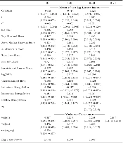
Table 4. Posterior Mean Estimates of Parameters across Models I–IV (cont.)

(I) (II) (III) (IV)

Mean of the log Lerner Index Constant –0.355 –0.714 –0.525

(–0.617; –0.188) (–1.414; –0.353) (–0.871; –0.212) t 0.044 0.032 0.030

(0.015; 0.055) (0.020; 0.048) (0.017; 0.055) t2

–0.004 –0.002 –0.001 (–0.008; –0.002) (–0.001; –0.003) (–0.012; 0.120) log(Size) 0.366 0.289 0.312

(0.216; 0.457) (0.155; 0.317) (0.181; 0.416) Top Hundred Bank 0.422 0.388 0.455

(0.289; 0.588) (0.101; 0.560) (0.317; 0.588) Asset Market Share in State 0.203 0.181 0.225

(0.113; 0.352) (0.044; 0.203) (0.141; 0.327) # Mergers in State 0.456 0.188 0.417

(0.382; 0.551) (0.072; 0.277) (0.226; 0.617) Securities Share 0.388 0.217 0.181

(0.144; 0.524) (0.044; 0.513) (0.072; 0.226) HHI for Loans 0.727 0.515 0.103

(0.551; 0.827) (0.313; 0.688) (0.064; 0.203) Non-interest Income Share 0.332 0.202 0.188

(0.187; 0.482) (0.103; 0.355) (0.065; 0.254) log(DPI) 0.316 0.217 –0.016

(0.188; 0.415) (0.188; 0.335) (–0.035; 0.044) Unemployment Rate 0.188 0.103 –0.022

(0.055; 0.213) (0.054; 0.210) (–0.036; –0.015) Intrastate Deregulation 0.316 –0.117 –0.025

(0.188; 0.440) (–0.221; –0.073) (–0.033; 0.015) Interastate Deregulation 0.283 0.132 –0.017

(0.155; 0.318) (–0.071; 0.218) (–0.022; 0.030) IBBEA Deregulation 0.187 0.351 –0.032

(0.133; 0.220) (0.144; 0.447) (–0.052; 0.071)

u1 0.228

(0.170; 0.316) Variance–Covariance

var(u1) 0.317 0.225 0.228 0.187 (0.285; 0.388) (0.188; 0.287) (0.186; 0.303) (0.115; 0.214) var(u2) 0.455 0.317 0.285

(0.388; 0.515) (0.289; 0.355) (0.212; 0.317) cov(u1, u2) 0.224

(0.216; 0.277)

Log Bayes Factor 22.351 1.000 2.305

differences in our formulation of the dependence between the cost efficiency and the Lerner index across specifications I through III also allow us to implicitly assess the underlying nature of the relationship between the two. Concretely, the log Bayes factors9 reported at the bottom of Table 4 indicate that our data distinctly favor the “agnostic” Model I over the two alternative econometric specifications of the joint dependence between uC and uL. Thus, the selected model implies that

the data are not revealing of a clear causal directionality in the relationship between the bank’s efficiency and monopolistic power.

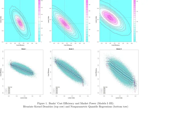
The QLH-consistent negative relationship between the bank’s cost efficiency and market power can be vividly seen by looking at Figure 1. The top row of Figure 1 depicts contours of bivariate kernel densities10 of the bank-level estimates of cost efficiency and the Lerner index for all three specification of our proposed model. These plots allow us to assess the relationship not just at a given moment (say, average) but distribution-wise. Conversely, plots in the bottom row of Figure 1 enable us to examine the relationship at different quantiles. Specifically, they show the estimated 10th, 25th, 50th, 75th and 90th quantiles of the bank’s cost efficiency conditional on its Lerner index. The fitted conditional quantile functions are obtained by inverting the nonparametrically estimated kernel conditional cdf of the cost efficiency given the market power.11 To avoid any confusion, we would like to stress that the plotted are not the confidence bounds. Both kinds of plots suggest that, when the simultaneous determination of the banks’ efficiency and the market power is modeled explicitly (as in Models I–III), the two exhibit a strong negative relationship. To the contrary of the above results from our system-based models, a single-equation Model IV points to a positive relationship between the bank’s cost efficiency and the Lerner index which is in line with the ESH. To see this, consider Figure 2 which plots the bivariate kernel density and the conditional quantile functions for the estimates from Model IV. For instance, Koetter et al. (2012) also find such a positive relationship using the method like the one of Model IV. However, since Model IV does not explicitly formulate the joint dependence between the market power and efficiency, we do not have a direct way to formally test for the sign of the relationship between the two. While one would normally be tempted to run a second-stage regression as widely done in the literature, the latter procedure would not produce valid inference in the light of the problems discussed in the Introduction. Thus, any inference, even informal, on the basis of patterns discernible from Figure 2 is likely to be misleading, especially because the estimates of both measures are prone to simultaneity and misspecification biases due to Model IV’s failure to meaningfully accommodate the joint dependence of the two.

We conclude by briefly commenting on the results pertaining to contextual controls. Most bank characteristics have significant effects on the mean cost inefficiency and marker power, and the effects are largely of expected signs with very few reversals across model specifications. We find that, over time, banks have generally acquired more market power while having become more cost inefficient. Rather expectedly, the results from all models also suggest that larger banks tend to be less efficient but also to exert greater monopolistic power in the markets than their smaller counterparts. Consistent with one’s intuition, the largest banks as well as, more generally, banks with larger market share are estimated to have more market power. Same holds for the institutions operating in less competitive markets as proxied by the number of mergers at the state level. The banks with higher market power are also found to be those with less diversified loan portfolios (higher HHI for loans) and those more heavily engaged in nontraditional activities. Based on the results from Model I most preferred by the data, we also find that the deregulation appears to have

9

Computed using a Laplace approximation (DiCiccio, Kass, Raftery & Wasserman, 1997). 10

We use an axis-aligned bivariate Gaussian kernel, evaluated on a square grid using the normal reference bandwidth. 11

Figure 1. Banks’ Cost Efficiency and Market Power (Models I–III):

Bivariate Kernel Densities (top row) and Nonparametric Quantile Regressions (bottom tow)

Figure 2. Bivariate Kernel Density and Nonparametric Quantile Regression of Banks’ Cost Efficiency and Market Power (Model IV)

positively contributed to the monopolization of the industry. The model also suggests that banks with lower z-scores (higher probability of insolvency) tend to be more cost inefficient.

5

Conclusion

This paper develops a novel unified econometric methodology for the formal examination of the market power – cost efficiency nexus. Our approach can meaningfully accommodate a mutually dependent relationship between the firm’s cost efficiency and marker power (as measured by the Lerner index) by explicitly modeling the simultaneous/endogenous determination of the two in a system of nonlinear equations consisting of the firm’s cost frontier and the revenue-to-cost ratio equation derived from its stochastic revenue function. Both the firm’s cost efficiency and marker power index are estimated jointly and derived from a single unified model thus enabling us to interpret and analyze them on a common ground. Our framework places no a priori restrictions on the sign of the dependence between the firm’s monopolistic power and efficiency as well as allows for different hierarchical orderings between the two, enabling us to meaningfully discriminate between competing quiet life and efficient structure hypotheses. Among other benefits, our approach completely obviates the need for second-stage regressions of the cost efficiency estimates on the constructed market power measures which, while widely prevalent in the literature, suffer from multiple econometric problems as well as lack internal consistency/validity.

for a simultaneous determination of the two. The latter highlights the pivotal importance of a proper econometric modeling of the market power – efficiency relationship which a popular two-stage analysis is unable to deliver.

Appendix: MCMC Techniques

Across all models (where appropriate), we use the following priors forγ₁,γ₂,ψ1,ψ1,ΩandΣ: γj ∼

N_(0,104_{I) for j= 1,2;ψj ∼}N_(0,104_{) independently for j= 1,2;p(Ω)∝ |Ω|}(−n¯+1)_{exp{tr[ ¯AΩ}−1_]}

and p(Σ) _{∝ |}Σ_|(−¯n+1)exp_{tr[ ¯AΣ−1]_}, both from the inverse-Wishart distribution with ¯n= 1 and ¯

A= 10−4_I.

A

Model I

The augmented kernel posterior distribution is

p(β,Σ,Ω,µ,u_|Ξ)_{∝ |}Ω_|−nT /2_|Σ_|−nT /2Φρ

Ω−_diag1 µ−nT_×

exp

(

−1₂

n X i=1 T X t=1 h

(rit−uit)′Σ−1(rit−uit)−(uit−µ)′Ω−1(uit−µ) i)

,

(A.1)

whererit=yit−

x′_itβ

f(xit;β)

.

Like we have showed in Section 3, while it is certainly possible to integrate the latent variables out, the resulting posterior is however highly nonlinear. Since β enters the second equation in (3.1) in a nonlinear way, we need to construct an efficient proposal distribution to use with the Metropolis-Hastings algorithm.

Let βb be some estimator of β, say, the least squares estimator applied to the cost function in (3.1a). Then, the scale elasticity can then be computed as P_mbεym,it = x′o,itRβb. Linearizing

f(xit;β) ≡ln P_mεym,it

, we obtain that fbit(x;β)≃ln P_mεbym,it

−1 + P_mbεym,it

−1

x′_o,itRβ. We next rewrite the system in (3.1) as follows:

y1,it−u1,it =x′itβ+v1,it (A.2a)

y2,it−ln

x′_o,itRβb+ 1₋u2,it ≃

R′xo,it

x′_o,itRβb−1 ′

β+v2,it ≡xe′o,itβ+v2,it. (A.2b)

For known values of uit, the GLS estimator ofβ is given by

β∗ =

n X i=1 T X t=1

XitΣ−1X′it !−1 _n

X

i=1

T X

t=1

XitΣ−1Yit, (A.3)

where we let Yit = "

y1,it−u1,it

y2,it−ln

x′_o,itRβb+ 1₋u2,it #

and Xit =

xit e

xo,it

. The corresponding GLS

variance-covariance matrix is V∗ =Pn_i=1P_tT₌₁XitΣ−1X′it −1

The proposal distribution is N_k(β∗_{, hV}∗_{), where h > 0 is a certain constant. If we draw a}

candidate βc _∼ N_k(β∗, hV∗) and the chain is currently at βo, according to the independence Metropolis-Hastings proposal, the acceptance probability is

min

(

1, exp

−12tr

Q(βc)Σ−1_−2h12 (βc−β∗)′V∗−1(βc−β∗)

exp₋1₂tr[Q(βo)Σ−1_]− 1

2h2 (βo−β∗)′V∗−1(βo−β∗) )

, (A.4)

whereQ(β) =Pn_i=1PT_t=1

yit−

x′_itβ

f(xit;β) yit−

x′_itβ

f(xit;β) ′

.

An alternative is to use a random walk Metropolis-Hastings proposal in whichβc _∼N_k(βo_{, hV}∗_).

The acceptance probability then becomes

min

(

1, exp

−12tr

Q(βc)Σ−1

exp₋1₂tr[Q(βo)Σ−1_]

)

. (A.5)

Also, note that the proposal distributions can be constructed using the direct least squares esti-mator of the cost function in (A.2a). In this case,β∗andV∗in the above discussion is to be replaced with β∗ = Pn_i=1PT_t=1xitx′it

−1_P

n i=1

PT

t=1xit(y1,it −u1,it) and V∗ =s2Pni=1

PT

t=1xitx′it −1

, wheres2 = (nT)−1Pn

i=1

PT t=1

y1,it−u1,it−xitβb 2

. Then, we can use either an independence or a random walk Metropolis-Hastings algorithm. The benefit is that we avoid the costly inversion of the GLS variance-covariance matrix in each MCMC iteration.

The posterior conditional distribution of uit is given by

p(uit|β,Σ,Ω,µ,Ξ)∝exp

−1₂(uit−µ∗it)′V−1(uit−µ∗it)

×✶(uit≥0), (A.6)

oruit|β,Σ,Ω,µ,Ξ ∼ N+_d (µ∗it,V). Random draws can be obtained, say, in the bivariate case by

using the conditional distributions as follows:

u1,it|u2,it,β,Σ,Ω,Ξ ∼ N+1 (bu1,it,1/V11)

u2,it|u1,it,β,Σ,Ω,Ξ ∼ N+1 (bu2,it,1/V22), (A.7)

where_bu1,it=µ∗1,it+V 12 V11

µ∗

2,it−u2,it

,u_b2,it=µ∗2,it+V 12 V22

µ∗

1,it−u1,it

,V−1 = [Vij; i, j= 1,2] and

µ∗_it=hµ∗

1,it, µ∗2,it i′

.

Since these distributions are univariate, we can use standard procedures for generating normal random variables truncated from below at zero. Here, we use the acceptance sampling based on an exponential distribution. For the truncated normal distribution u _∼N+_{(M, v), the parameter}

of the exponential distribution is λ = M+√M₂ 2+4v. The draw u _∼ E_{xp(λ) is accepted with the}

probability

exp

λu₋1₋ 1

2v(u−M)

2_{+ λ}−1

−M2

, (A.8)

which corresponds to the unique solution of the saddle-point problem:

min

λ maxu :λ

−1_expλu

− ₂1_v(u₋M)2

The analogous problem in the multivariate caseu_∼N+

d (M,V) has the solutionλ+V−1M−

V−1Λ−1 = 0d, where Λ = diag{λ} = diag{λ1, ..., λm} is the matrix of the parameters of the

exponential distributions. Assuming λ1 = · · · = λm = α, the unique solution is given by α =

d−1Pd i=1u∗i

−1

, whereu∗ solves the following equations:

1d=d 1′du∗

V−1(u∗₋M). (A.10) Next, the posterior conditional distribution of Σis given by

p(Σ_|β,Ω,u,Ξ)_{∝ |}Σ_|−nT /2exp

−1₂trA∗Σ−1

, (A.11)

whereA∗=Pn_i=1PT_t=1(rit−uit) (rit−uit)′, i.e., a Wishart distribution.

Further, the posterior conditional distribution of Ω−1 is

p Ω−1_|β,Σ,u,µ,Ξ_{∝ |}Ω_|−nT /2exp

−1

2tr

A∗∗Ω−1

Φρ

Ω−_diag1 µ−nT, (A.12)

where A∗∗ = Pn_i=1PT_t=1(uit−µ) (ui−µ)′, which would have been a Wishart distribution if it

were not for the last term. Finally, we have

p(µ_|β,Σ,Ω,u,Ξ)_∝exp

−1₂trΩ−1A∗∗

Φρ

Ω−_diag1 µ−nT, (A.13)

from where it follows thatµ_|β,Σ,Ω,u,µ,Ξ _∼ N_d(nT)−1Pn

i=1

PT

t=1uit, (nT)−1Ω

, apart from the last term in the above expression.

We note that, if the location parameter of the truncated normal distribution ofuitis not constant

but varying with some contextual variables, i.e., ifµit=

µ1,it

µ2,it

=

z′_1,itγ₁

z′_2,itγ₂

=

z1,it 0l1

0_l2 z2,it ′_γ

1

γ₂

≡

Z′_itγ, where z1,it and z2,it is an l1×1 and l2×1 vector of covariates, andγ1 and γ2 is an l1×1

and l2×1 vector of the corresponding parameters, respectively, then

p(γ_|β,Σ,Ω,u,Ξ)_∝ exp

(

−1₂trΩ−1

n X i=1 T X t=1

uit−Z′itγ

uit−Z′itγ ′ ) × n Y i=1 T Y t=1 Φρ

Ω−_diag1 Z′_itγ−1. (A.14)

From the first half of the above expression it follows that γ_|β,Σ,Ω,u,Ξ _∼ N_l

1+l2(γb,Vγ),

where γ_b = Z′ InT ⊗Ω−1Z−1Z′ InT ⊗Ω−1U and Vγ = Z′ InT ⊗Ω−1Z−1 with U =

[u1,11, . . . , u1,nT, u2,11, . . . , u2,nT]′ and

Z=          

z′_1,11 0

..

. ...

z′_1,nT 0

0 z′_2,11

..

. ...

0 z′_2,nT

being of the 2nT _×1 and 2nT _×(l1 +l2) dimensions, respectively. Apart from the nonlinear

product term appearing in the second half of the expression in (A.14), the posterior conditional corresponds to the SUR model. Hence, for samples of the large size, γ_b can be computed as γ_b =

Pn i=1

PT

t=1ZitΩ−1Z′it −1_P

n i=1

PT

t=1ZitΩ−1Uit along with Vγ =Pni=1

PT

t=1ZitΩ−1Z′it −1

.

B

Model II

Since, in our empirical application, we setz1,it=z2,it =1, t,1₂t2′, here we focus on the special case

whenz1,it=z2,it ≡zit, which is said to be of dimensionl. When estimating the hierarchical model,

the only component which changes in the MCMC scheme is the way we sample the latent variables and their corresponding parameters. After some algebra in the kernel posterior distribution, we derive the following posterior conditional distributions:

uit|β,γ, ψ1,Σ, ω12, ω22,Ξ ∼ N+2 (ubit,Vu)×Φ z′itγ1+ψ1u2,it/ω1−1, (B.1)

where

b

uit= ω12ω22Σ−1+ ω12+ω22 1 +ψ21

I2− 1

ω₁2ω₂2Σ−1rit+ [ι2⊗zit]′ϕ

ϕ=

γ₁/ω2₂ ω2

1 γ2−ψ1ω22γ1

Vu=ω21ω22 Σ−1+ ω21+ω22 1 +ψ12

I2−1,

whereι2 is a 2×1 vector of ones.

Sinceu2,it appears in a nonlinear way, we can use the following alternative posterior conditional

distributions:

u1,it|u2,it,β,γ, ψ1,Σ, ω21, ω22,Ξ ∼ N+

µ1,it,

ω₁2

1 +σ11ω12

(B.2a)

u2,it|u1,it,β,γ, ψ1,Σ, ω21, ω22,Ξ ∼ N+

µ2,it,

ω₂2

1 +σ22ω22

×Φ z′_itγ₁+ψ1u2,it/ω1−1, (B.2b)

where

µ1,it =

ψ1−ω12σ12u2,it+z′itγ1+ω12 Σ−1rit₁

1 +σ11ω21

, µ2,it= −

ω₂2σ12u1,it+z′itγ2+ω22 Σ−1rit₂

1 +σ22ω22

and Σ−1rit_j denotes thejth row of Σ−1ritforj= 1,2. Although the first conditional

distribu-tion above is a truncated normal, the second one is however not due to the presence of its last term, which comes from the normalizing constant of the prior conditional foru1,it|u2,it,zit. To draw

sam-ples from this conditional distribution, we first write it in the form ofx_∼N+ _{µ, v}2_{×Φ (a+bx)}−1

using obvious notation. Suppose w = a+ bx. It is then easy to show that the derivatives of the log density are f′_{(x) =} 1

2(bv)−1(w −a−bµ) + bvΛ(w), where Λ(w) = φ(w)/Φ(w) and

−f′′_{(x) =} 1

2+ (bv)2Λ(w) [1 + Λ(w)]>0 for allw∈R, from where it follows that the distribution is

log-concave. The mode satisfies the following nonlinear equation: w∗_{+ 2(bv)}2_Λ(w∗_{)−(a+bµ) = 0,}

from where we get x∗ _{= b}−1_(w∗_{−a). Thus, we can use acceptance sampling when the source}

distribution is x_∼N+_x∗_,−f′′_(x∗₎−1_.

is one fixed-point iteration away from the initial conditionw(0) _{=a+bµ. Second, in extreme cases}

when it takes more than 100 rejections to obtain a draw, we resort to a Metropolis-Hastings by drawingx_∼N+_a−1_(w∗_−b),−f′′ _a−1_(w∗_−b)−1_{and accepting the draw with the probability}

min

1, exp

−₂1_v2

(x₋µ)2+x(o)₋µ2

+_2v12

(x₋x∗)2+x(o)₋x∗2

Φ (a+bx)−1Φa+bx(o).

(B.3) For other parameters, the posterior conditional distributions are as follows:

γ₁

ψ1

uit,β,γ2,Σ, ω12, ω22,Ξ ∼ Nl+1

Z′_uZu−1Z′uu1, ω12 Z′uZu−1 × n Y i=1 T Y t=1

Φ z′_itγ₁+ψ1u2,it/ω1−1

(B.4a)

γ_2|uit,β, ψ1,Σ, ω12, ω22,Ξ ∼ Nl Z′Z)−1Z′u2, ω22(Z′Z)−1

× n Y i=1 T Y t=1

Φ z′_itγ₂/ω2−1, (B.4b)

whereZ= [z11, . . . ,znT]′,u1= [u1,11, . . . , u1,nT]′,u2 = [u2,11, . . . , u2,nT]′ andZu =Z u2.

C

Model III

Similar to Model II, here we focus on the special case when z1,it = z2,it ≡ zit, which is said to

be of dimension l. If approximations to the marginal distributions are available, then the joint distribution of u1,it and u2,it is

e

p(u1,it, u2,it|zit) = h

p(u1,it|u2,it,zit)p(u2,it|u1,it,zit)pe(u1,it|zit)pe(u2,it|zit) i1/2

, (C.1)

where p_e(u1,it|zit) and pe(u2,it|zit) denote certain approximations to the marginal distributions.

Specifically, we use the following approximations:

u1,it|zit ∼ N+ µb1,it, ωb12

(C.2a)

u2,it|zit ∼ N+ µb2,it, ωb22

, (C.2b)

where the location and scale parameters are to be determined. To build such approximations, we use MCMC to obtain a large sample of dependent draws

u_it(s) =hu₁(s_,it), u(₂s_,it)i′, s= 1, ..., S

from the specification of conditional distributions. Therefore, the posterior distribution of the latent variables is

p(u₁,it, u₂,it|Ξ,θ) = exp

−1

2(uit−rit)

′_Σ−1_(u it−rit)

×

h

p(u1,it|u2,it,zit)p(u2,it|u1,it,zit)pe(u1,it|zit)pe(u2,it|zit)

i1/2

∝exp

−1₂(uit−rit)′Σ−1(uit−rit)− 1 4ω2

1

(u₁,it−z′itγ1−ψ1u2,it)2− 1 4ω2

2

(u₂,it−z′itγ2−ψ2u2,it)2

×

Φ−1/2_((z′

itγ1+ψ1u2,it)/ω1) Φ−1/2((z′itγ2+ψ2u1,it)/ω2)×

exp

− 1 4ωb2

1

(u₁,it−µb1,it)2− 1 4ωb2

2

(u₂,it−µb2,it)2