Enhanced Structural Complexity Index: An Improved Index for Describing Forest Structural Complexity

Published Online January 2013 in SciRes (http://www.scirp.org/journal/ojf) http://dx.doi.org/10.4236/ojf.2013.31005

Enhanced Structural Complexity Index: An Improved Index for

Describing Forest Structural Complexity

Philip Beckschäfer

_{, Philip Mundhenk}

_{, Christoph Kleinn}

_{, Yinqiu Ji}

_,

Douglas W. Yu

_{, Rhett D. Harrison}

1_{Chair of Forest Inventory and Remote Sensing, Georg-August-Universität Göttingen, Göttingen, Germany} 2_{State Key Laboratory of Genetic Resources and Evolution, Kunming Institute of Zoology, Chinese Academy of}

Sciences, Kunming, China

3_{School of Biological Sciences, University of East Anglia, Norwich, UK}

4_{Key Laboratory for Tropical Forest Ecology, Xishuangbanna Tropical Botanical Garden, Chinese Academy of}

Sciences, Menglun, China Email: [email protected]

Received November 19th_{, 2012; revised December 19}th_{, 2012; accepted December 30}th_{, 2012}

The horizontal distribution of stems, stand density and the differentiation of tree dimensions are among the most important aspects of stand structure. An increasing complexity of stand structure is often linked to a higher number of species and to greater ecological stability. For quantification, the Structural Com- plexity Index (SCI) describes structural complexity by means of an area ratio of the surface that is gener- ated by connecting the tree tops of neighbouring trees to form triangles to the surface that is covered by all triangles if projected on a flat plane. Here, we propose two ecologically relevant modifications of the SCI: The degree of mingling of tree attributes, quantified by a vector ruggedness measure, and a stem density term. We investigate how these two modifications influence index values. Data come from forest inventory field plots sampled along a disturbance gradient from heavily disturbed shrub land, through secondary regrowth to mature montane rainforest stands in Mengsong, Xishuangbanna, Yunnan, China. An application is described linking structural complexity, as described by the SCI and its modified ver- sions, to changes in species composition of insect communities. The results of this study show that the Enhanced Structural Complexity Index (ESCI) can serve as a valuable tool for forest managers and ecolo- gists for describing the structural complexity of forest stands and is particularly valuable for natural for- ests with a high degree of structural complexity.

Keywords: Forest Structure Index; Structural Complexity; Stem Map; Species Composition; NMDS

Introduction

The importance of ecosystem structure to species richness has been established through many studies. Already in the early 1960s MacArthur and MacArthur (1961) showed that the physi- cal structure of a plant community was of greater importance than the composition of plant species in determining bird diver- sity. A meta-analysis by Tews et al. (2004) found that 85% of 85 reviewed studies on habitat heterogeneity and species rich- ness conducted between 1960 and 2003 found a positive corre- lation between richness and structural variables. As plants play an important role in shaping the physical structure of many environments (Lawton, 1983; McCoy & Bell, 1991) the struc- tural complexity of plant communities has frequently been used as an indicator of the diversity in other taxa (Whittaker, 1972; Franzreb, 1978; Temple et al., 1979; Aber, 1979; Recher et al., 1996; Moen & Gutierrez, 1997). Moreover, the habitat hetero- geneity hypothesis (Simpson, 1949; MacArthur & Wilson, 1967) relates this positive association between species diversity and structural complexity by suggesting that more complex environments provide increased niche space and thus facilitate specialization and avoidance of competition through spatial segregation (Cramer & Willig, 2005). This further implies that the structural complexity of a forest is of great importance for the number and composition of species inhabiting it (Willson,

1974; Ambuel & Temple, 1983; Freemark & Merriam, 1986; Spanos & Feest, 2007).

the spatial arrangement of plant dimensions, both horizontally and vertically (Zenner & Hibbs, 2000).

Several indices have been developed in the past decades to provide interpretable metrics of structural complexity and thus facilitate comparisons among stands (Pommerening, 2002; LeMay & Staudhammer, 2005; McElhinny, 2005). LeMay & Staudhammer (2005) identify three groups of indices: 1) indices based on tree attributes, 2) indices of spatial heterogeneity and 3) indices combining tree attributes and spatial heterogeneity. While indices in groups 1) and 2) focus on only one aspect of forest structural complexity, indices in group 3) intend to retain more information and thus may provide more comprehensive measures of structural complexity.

In this study we propose an index that integrates the hori- zontal distribution of trees, stand density, and the differentiation and intermingling of tree dimensions into one measure, while requiring only data on tree position and diameter-at-breast- height (DBH) for its calculation. Our index is a modification of

the Structural Complexity Index (SCI) developed by Zenner &

Hibbs (2000). In the first part of this study, we describe limita- tions of the SCI and propose two modifications to create an

Enhanced Structural Complexity Index (ESCI). In the second

part, the SCI and ESCI are calculated for forest inventory data from an upland landscape in Xishuangbanna, South China, and results are compared. In the last part, we compare how the SCI

and ESCI correlate with turnover in insect species composition.

The Structural Complexity Index (

SCI

)

Zenner & Hibbs (2000) introduced the SCI, a formula that

mathematically integrates both vertical (size differentiation) and horizontal (spatial position) components of forest structure. It is based on the position of trees whose xy-coordinates are complemented with a tree attribute, such as DBH or height, as a

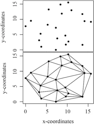
z-coordinate. By a spatial tessellation approach (Delaunay, 1934) each tree is connected to its neighbours such that train- gles are defined that form a continuous faceted surface, i.e. a triangulated irregular network (TIN) (Figure 1). If tree height is

selected as the z-coordinate, this TIN can be visualized as con-

necting the tops of neighbouring trees. Instead of tree height, any measured continuously or ordinally scaled tree attribute can be chosen as the z-coordinate. The SCI is defined as the surface

area of the TIN in three dimensional space divided by the area covered by its projection on a plane surface (Equation (1)). If all trees have the same z-value (e.g. all trees have the same height

or basal area as in an even aged plantation) the SCI equals 1,

the lower limit of the SCI. For structurally more complex forest

stands the SCI is >1.

surface area of TIN projected area of TIN

SCI

Limitations of the

SCI

We illustrate basic characteristics of the SCI with a set of four simple forest stands which differ in their structural com- plexity but have the same SCI value. All stands cover the same

area but vary in number of trees, range of tree height, and spa- tial mingling of trees with different heights (Table 1, Figure 2). Observe that a stand composed of 36 regularly planted trees with a range of tree heights between 14 and 18 meters (Figure 2(a)) has the same SCI value as a stand with 8 trees and a range

of tree heights between 1 and 12 meters (Figure 2(c), Table 2).

Intuitively, these two stands have very different structures, and it may be considered an undesirable property of the SCI that it

is not able to differentiate these stands.

Figure 1.

Spatial distribution of stems (upper panel). Tri- angulated irregular network calculated for stems in the upper panel (lower panel).

Table 1.

Stand characteristics of example forest stands from Figure 2.

Stand Area _[m²] No. of _trees Range of tree _{heights [m] height [m]} Mean tree

Standard deviation of tree heights

No. of individual

heights

a) 1600 36 14 - 18 16.0 2.03 2

b) 1600 36 1 - 21 11.0 6.92 6

c) 1600 8 1 - 12 7.03 5.38 3

d) 1600 14 1 - 21 10.0 8.55 5

(a) (b)

(c) (d)

Figure 2.

Table 2.

Structural Complexity Index (SCI) and Enhanced Structural Complex- ity Index (ESCI’ and ESCI) values of example stands from Figure 2

and Table 1.

Stand SCI ESCI’ ESCI TIN area [m²] projected area [m²] VRMTrees/10 m2

a) 1.17 1.33 1.63 1295.77 1111.11 1.14 .23 b) 1.17 1.17 1.43 1295.77 1111.11 1.00 .23

c) 1.17 1.33 1.40 1295.77 1111.11 1.15 .05 d) 1.17 1.17 1.27 1295.77 1111.11 1.00 .09

The Enhanced Structural Complexity Index

(

ESCI

)

We propose two modifications to the SCI to avoid the ambi-

guity described above and to better distinguish specific proper- ties of structural complexity.

The two proposed modifications of the SCI towardsthe En-

hanced SCI (ESCI) are:

1) Incorporation of triangle orientations;

2) Incorporation of triangle orientations + stem density. The first modification enables the index to distinguish forest type a from type b, as in Figure 2. The two types do not differ

in stem density, and trees in both stands are located on a regular grid with a spacing of 4 m. However, they differ in the range of tree heights and in the mingling of tree dimensions. In forest type b, there is a clear trend from small trees in the first row towards larger trees in the last row. This can be imagined as a forest edge in which tree height gradually increases towards the forest interior or as adjacent strips of clear cuts, each at a dif- ferent age. In contrast, forest type a is composed of only two distinct tree heights; rows of 14 m high trees alternate with rows of 18 m high. The resulting TINs have the same surface area for both stands, resulting in the same SCI value.

To distinguish between these stand types, the orientation of triangles in the TINs is quantified by a vector ruggedness measure (VRM) (Equation (3)), adapted from a method pro- posed by Hobson (1972) and Sappington et al. (2007). Here, unit vectors are used to represent the orientation of a triangle (Figure 3). To centre a unit vector at triangle i, the cross prod-

uct of triangle sides ai and bi is calculated. This results in a

vector that is divided by its own length to standardize length to one. To ensure that all unit vectors are oriented upwards, unit vectors with a negative z-coordinate are mirrored. All unit vec-

tors are summed, resulting in a new vector whose strength (VSTR, Equation (2)) is divided by the number of triangles in

the TIN (n) and subtracted from 2 (Equation (3)). The resulting VRM is a dimensionless measure that ranges from 1 (non-rug-

ged) to 2 (most rugged).

The ESCI’ is calculated by multiplying the SCI with the VRM (Equation (4)). Based on the ESCI’ forest types a (ESCI’

= 1.6) and b (ESCI’ = 1.3) can clearly be distinguished (see

Table 2).

1

n

i i

i i i

a b VSTR

| a b |

  





2 VSTR

VRM

n

  (3)

ESCI 'SCI * VRM (1)

The second modification enables one to discriminate among forest types a and c and types b and d (Figure 2). Compared to

forest types a and b, types c and d contain fewer trees (8 and 12 trees respectively) and cover different height ranges (Table 1).

Since stem density is considered an important structural characteristic (e.g. Pretzsch, 2009), the number of stems per unit area is included in the ESCI by multiplying the number of

stems per 10 m2 _{with the ESCI’(Equation (5)). Hence, the}

in-dex calculated for stands with low stem densities is lower than for stands with high stem densities. To avoid too much weight being assigned to the stem density, a value of 1 is added to the number of stems per 10 m2_{. The ESCI is a dimensionless meas-}

ure >1 that increases with stem density, the intermingling of trees with different attributes, and differences between tree at- tributes.





ESCIESCI '*  (5)

Case Study from Mengsong, Xishuangbanna,

Yunnan, China

Data Collection and Analysis

To investigate the ESCI and the ESCI’ compared to the SCI,

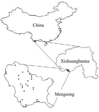
these indices were calculated for 28 plots of a forest inventory carried out in Mengsong township, Xishuangbanna, Yunnan, China (UTM/WGS84: 47 N 656355 E, 2377646 N, alt = 1600 m) (Figure 4). Plots cover the study site along a disturbance gra-

dient from heavily disturbed shrub land, through secondary re- growth to mature montane rainforest stands. Each plot consists of nine circular 10 m-radius sub-plots (314.16 m2_{) arranged on}

(a)

(b)

Figure 3.

China

Xishuangbanna

Mengsong

Figure 4.

Location of the study site Mengsong in Xishuang-banna, China. Black squares show plot locations within the site.

a square grid with 50 m spacing (Figure 5). For sub-plots lar-

ger 250 m2_{, mean and median}

SCI values have been shown to

be scale-invariant (Zenner, 2005).

In each sub-plot, DBH and position (azimuth and distance to

sub-plot centre) were recorded for all trees with a DBH≥ 10 cm. SCI, ESCI’, and ESCI were calculated for each sub-plot using

basal area of each tree as the z-coordinate. Sub-plots without at least three trees were assigned SCI, ESCI’ and ESCI values of

zero. The R statistical software (R Core Team, 2012) and the geometry package (Grasman et al., 2011) were used for the

Delaunay triangulation. Per plot values were derived by aver- aging all 9 sub-plot values per plot.

In five sub-plots (No. 1, 3, 5, 7, 9) per plot, insects were col- lected using Malaise traps in April-May 2011. Malaise traps were left in place for one week per plot and for each plot, spe- cies composition was determined using high-throughput DNA metabarcoding of the cytochrome oxidase subunit I (COI) bar- code gene (Yu et al., 2012). Insect species were approximated with 97% threshold-similarity Operational Taxonomic Units (OTUs), each representing a cluster of similar COI sequences.

Insect community composition was examined by non-metric multidimensional scaling (NMDS) (Legendre & Legendre, 1998; Quinn & Keough, 2002). NMDS maps the position of plots in species space, in our case represented by the Jaccard dissimilarities of Hellinger transformed per plot OTU counts (Yu et al., 2012), onto a predefined number of axes in an itera- tive search for an optimal solution. NMDS is commonly re- garded as the most robust unconstrained ordination method in community ecology (Minchin, 1987). The R package vegan

(Oksanen et al., 2007) was used for the ordination analysis. To investigate whether a relationship exists between structural complexity and turnover in insect species composition we used the function envfit in the package vegan to calculate the fit of

environmental variables to the ordination scores. envfit maxi-

mises the correlation of environmental variables to the matrix of ordination scores and uses a permutation test to evaluate the probability of obtaining the resulting or a higher r2value. P-

values stated here are based on 1000 permutations. To test whe- ther differences in correlation coefficients between SCI, ESCI’

and ESCI are significant we took 1000 subsamples (without

replacement) of 26 observations from our field data. NMDS ordinations were calculated for each subsample and the corre- sponding r² values with SCI, ESCI’ and ESCI were calculated. Subsequently, we applied Mann-Whitney U tests to investigate

whether differences of mean r² values of the replicated samples

were significant.

Results

From a total of 2890 trees that were recorded, each sub-plot contained on average 11.47 trees, with numbers ranging from 0 to 34 trees per sub-plot. The basal area of individual trees var- ied from 78.61 cm2 _{to 11,750 cm}2_.

Across all sub-plots, ESCI values are consistently higher and

cover a larger range than do ESCI’ values. The same is ob-

served if ESCI’ and SCI are compared (Figure 6).

In addition to the observed differences in index value range, the indices treat special cases of tree arrangements differently. For example, sub-plots 49_2 and 372_9 (Figure 7, upper panels)

have similar SCI values (1% difference), but their ESCI’ values

differ substantially (22.75% difference) (Table 3). However, in

Figure 7, sub-plots 49_2 and 90_1 still have similar structural

complexities, as measured by the ESCI’.

Figure 5.

Plot design: Cluster plot consisting of 9 sub-plots arranged on a square grid with 50 meters spacing between sub- plot centres.

Figure 6.

Figure 7.

Depiction of tree positions (xy-coordinates; in meters) complemented with basal area (BA) as the z-coordinates of sub-plots listed in Table 3. Upper panels: Sub-plot 49_2 has a SCI value similar to sub-plot 372_9. Based on the ESCI’ value 49_2 is similar to 90_1. Lower panels: Sub-plots with similar ESCI’ values which would be distinguished by their ESCI values. Note: ESCI ranks the sub-plots in a different order than SCI.

Table 3.

Index values calculated for sub-plots shown in Figure 7.

sub-plot projected area [m²]

TIN area

[m²] SCI ESCI’ ESCI VRM No. of

trees 49_2 47.53 24911.01 524.15 528.26 595.51 1.01 4 372_9 222.35 119133.61 535.79 1014.81 1790.07 1.89 24

90_1 113.11 33290.73 294.31 532.38 667.95 1.81 8

189_9 36.94 40896.36 1107.08 1445.78 1629.86 1.31 4

398_3 43.86 40417.48 921.44 1452.41 1729.81 1.58 6 192_8 166.83 133784.66 801.91 1473.12 2551.62 1.84 23

The effect of the incorporation of the stem density term be- comes clear when the sub-plots in Figure 7 (lower panels) are examined. According to their SCI values, sub-plot 189_9 has a

higher structural complexity than does 398_3 or 192_8. ESCI

ranks sub-plot 189_9 as the least structurally complex and 192_8 as the most structurally complex (Table 3).

The number of NMDS dimensions was fixed to three after visual examination of the scree plot of stress vs dimensions. Three dimensions provided a satisfactory stress value of 9.24%. There were highly significant (p < .001) correlations between all three structural complexity indices and the NMDS ordina- tion. The SCI shows the lowest r2 value of .51 followed by the ESCI’ with r2 = .54 and ESCI with r2 = .59. Mean r2 values

based on 1000 sample replicates were significantly different among all combinations of indices (p < .0001).

Discussion

The number of stems per 10 m2 _{is a critical factor in the}

ESCI formula. In the data set used in this study, we found that (1 + No. of stems per m²) results in a range of values from 1 to

2.02, for 0 and 32 trees per sub-plot respectively. This range does not assign a weight to the number of stems that outweighs the other terms of the equation. SCI, VRM and stem density are

hence of approximately equivalent importance in determining the ESCI value. For other data sets with a higher number of

stems per unit area, the relation to the base of 10 m2 _probably

leads to density values that dominate the resulting ESCI value.

A higher stem density might occur, for example, in different forest types, succession stages with high stem numbers, or if the DBH threshold is lower than 10 cm. In these cases it might

be more informative to calculate ESCI’ and stem density sepa-

rately to describe structural complexity and to make inferences. The addition of 1 to the number of stems per 10 m2 _{assigns a}

greater weight to low stem densities but has little influence if stem densities are high. This weighting takes into account that with increasing density, the potential for a spatial differentia- tion decreases.

Sub-plots in which stems were mapped for this analysis cover an area of 314.16 m2_{, which is sufficiently large for the}

calculation of the SCI (Zenner, 2005). Nevertheless, due to the high scale dependency of forest structure (Franklin et al., 2002; Zenner, 2005), this plot size is probably at the lower bound of an adequate size. A further investigation of the variability of

ESCI’ and ESCI values at varying scales is recommended to achieve deeper insights regarding the minimum plot size for calculations of these indices.

In the structural assessment of forests, the inclusion of small diameter trees was found to enhance the detection of structure types (Zenner et al., 2011). In future studies it might be inter- esting to analyse whether ESCI’ and ESCI show a similar re-

sponse if trees with a DBH < 10 cm are considered.

Comparing SCI, ESCI’ and ESCI, we find that the stronger emphasis on the intermingling of tree dimensions through the incorporation of the VRM as a measure of surface ruggedness

improves the ability of the indexto discriminate among stand conditions. This might result in a better utility of the index. For example, it could be used for a separation of forest edges with increasing tree height from other spatial arrangements of tree dimensions typical for forest interiors. Such discrimination makes sense from an ecological point of view since forest edges are characterized by a distinct microclimate and resource spec- trum, with corresponding effects on species composition and abundance (McDonald & Urban, 2006). If in addition to the

VRM, the stem density of a forest is taken into account, the

ability to unambiguously characterize forest structural comple- xity is increased again. Ecologists and forest managers likewise consider stem density as an important aspect of structural com-plexity because it determines the mean growing space per plant and hence is an indicator of competition for resources within the stand (Pretzsch, 2009). Changing stem density is the princi- pal way forest managers manipulate forests (Davis et al., 2001), and these changes alter forest habitats with consequences for forest organisms.

A possible ecological relevance of the modifications of the

SCI is indicated by the correlation of the index values with the

NMDS ordination, which describes turnover in insect species composition. Compared to the SCI, significantly stronger corre-

lations with the NMDS ordination were observed for the ESCI’

and the ESCI. The observed correlations support the habitat he-

these indices perform at least as well and possibly better in de- tecting this relationship. Nevertheless, the increase in r2 values

was only moderate, and hence it would be valuable to test the indices for structural complexity against other data sets from different geographic regions and taxa and to assess associations at multiple spatial scales.

Conclusion

The results of this study show that the suggested modifica- tions to the SCI are valuable improvements that increase the

ability to characterize the structural complexity of forests.

ESCI’ and ESCI allow for a more complete view of a forest

structure than the SCI. This makes these indices relevant to ecologists, forest scientists, and forest managers who are inter- ested in the relationship between ecosystem structure and bio- diversity.

Acknowledgements

Above all, we are indebted to the Advisory Group on Inter- national Agricultural Research (BEAF) at the German Agency for International Cooperation (GIZ) within the German Minis- try for Economic Cooperation (BMZ) for funding this research (project number 08.7860.3-001.00 “Making the Mekong Con- nected”—MMC). We are grateful to all members of the MMC-project for excellent support in coordinating and imple- menting research and field work, and in particular to the head of the project Prof. Dr. Xu Jianchu and the “various fathers” of the project including Dr. Horst Weyerhäuser and Dr. Timm Tennigkeit.

REFERENCES

Aber, J. (1979). Foliage-height profiles and succession in northern hardwood forests. Ecology, 60, 18-23.

doi:10.2307/1936462

Ambuel, B., & Temple, S. (1983). Area-dependent changes in the bird communities and vegetation of southern Wisconsin forests. Ecology, 64, 1057-1068. doi:10.2307/1937814

Cramer, M., & Willig, M. (2005). Habitat heterogeneity, species diver- sity and null models. Oikos, 108, 209-218.

doi:10.1111/j.0030-1299.2005.12944.x

Davis, L., Johnson, K., Bettinger, P., & Howard, T. (2005). Forest management—To sustain ecological, economic, and social values. Prospect Heights: Waveland Press, Inc.

Doherty, M., Kearns, A., Barnett, G., Sarre, A., Hochuli, D., Gibb, H., & Dickman, C. (2000). The interaction between habitat conditions, ecosystem processes and terrestrial biodiversity: A review. State of the Environment, Second Technical Paper Series (Biodiversity), En- vironment Australia, Department of Environment and Heritage. Franklin, J., Spies, T., Pelt, R., Carey, A., Thornburgh, D., Berg, D. et

al. (2002). Disturbances and structural development of natural forest ecosystems with silvicultural implications, using Douglas-fir forests as an example. Forest Ecology and Management, 155, 399-423. doi:10.1016/S0378-1127(01)00575-8

Franzreb, K. (1978). Tree species used by birds in logged and unlogged mixed-coniferous forests. The Wilson Bulletin, 90, 221-238. Freemark, K., & Merriam, H. (1986). Importance of area and habitat

heterogeneity to bird assemblages in temperate forest fragments. Biological Conservation, 36, 115-141.

doi:10.1016/0006-3207(86)90002-9

Grasman, R., Gramacy, R.B., & Sterratt, D. C. (2011). Geometry: Mesh generation and surface tesselation. R Package Version 0.2-0. URL (last checked 5 June 2012).

http://CRAN.R-project.org/package=geometry

Kimmins, J. (2005). Forest ecology: A foundation for sustainable forest management and environmental ethics in forestry (3rd ed.). Upper Saddle River, NJ: Prentice Hall.

Lawton, J. (1983). Plant architecture and the diversity of phytophagous insects. Annual Review of Entomology, 28, 23-39.

doi:10.1146/annurev.en.28.010183.000323

Legendre, P., & Legendre, L. (1998). Numerical ecology. Elsevier Sci- ence & Technology, 20, 853.

LeMay, V., & Staudhammer, C. (2005). Indices of stand structural diversity: Mixing discrete, continuous, and spatial variables. In Pro- ceedings of the IUFRO Sustainable Forestry in Theory and Practice: Recent Advances in Inventory & Monitoring, Statistics, Information & Knowledge Management, and Policy Science Conference (p. 4). Edinburgh, 5-8 April 2005.

MacArthur, R., & MacArthur, J. (1961). On bird species diversity. Ecology, 42, 594-598. doi:10.2307/1932254

MacArthur, R., & Wilson, E. (1967). The theory of island biogeogra- phy. Princeton, NJ: Princeton University Press.

McCoy, E., & Bell, S. (1991). Habitat structure: The evolution and di- versification of a complex topic (pp. 3-27). London: Chapman and Hall.

McDonald, R., & Urban, D. (2006). Edge effects on species composi- tion and exotic species abundance in the North Carolina piedmont. Biological Invasions, 8, 1049-1060. doi:10.1007/s10530-005-5227-5 McElhinny, C., Gibbons, P., Brack, C., & Bauhus, J. (2005). Forest and

woodland stand structural complexity: Its definition and measure- ment. Forest Ecology and Management, 218, 1-24.

doi:10.1016/j.foreco.2005.08.034

Minchin, P. (1987). An evaluation of the relative robustness of tech- niques for ecological ordination. Plant Ecology, 69, 89-107. doi:10.1007/BF00038690

Moen, C., & Gutierrez, R. (1997). California spotted owl habitat selec- tion in the central Sierra Nevada. The Journal of Wildlife Manage- ment, 61, 1281-1287. doi:10.2307/3802127

Oksanen, J., Kindt, R., Legendre, P., O’Hara, B., Stevens, M., Oksanen, M., & Suggests, M. (2007). The vegan package. Community ecology package. URL (last checked 5 June 2012).

http://www.R-project.org

Polley, H. (2007). Survey instructions for federal forest inventory II (2001-2002), 2nd corrected translation, February 2006, of the 2nd corrected and revised reprint, May 2001. Federal Ministry of Food, Agriculture and Consumer Protection, Bundesministerium für Ver- braucherschutz, Ernährung und Landwirtschaft (BMVEL). URL (last checked 10 September 2012).

http://www.bundeswaldinventur.de/media/archive/513.pdf

Pommerening, A. (2002). Approaches to quantifying forest structures. Forestry, 75, 305-324. doi:10.1093/forestry/75.3.305

Pretzsch, H. (1997). Analysis and modeling of spatial stand structures. Methodological considerations based on mixed beech-larch stands in Lower Saxony. Forest Ecology and Management, 97, 237-253. doi:10.1016/S0378-1127(97)00069-8

Pretzsch, H. (2009). Forest dynamics, growth and yield: From meas- urement to model. Berlin: Springer Verlag.

Quinn, G., & Keough, M. (2002). Experimental design and data analy- sis for biologists. Cambridge: Cambridge University Press. doi:10.1017/CBO9780511806384

R Core Team (2012). R: A language and environment for statistical computing. Vienna: R Foundation for Statistical Computing. Recher, H., Majer, J., & Ganesh, S. (1996). Eucalypts, arthropods and

birds: On the relation between foliar nutrients and species richness. Forest Ecology and Management, 85, 177-195.

doi:10.1016/S0378-1127(96)03758-9

Sappington, J., Longshore, K., & Thompson, D. (2007). Quantifying landscape ruggedness for animal habitat analysis: A case study using bighorn sheep in the Mojave Desert. The Journal of Wildlife Man- agement, 71, 1419-1426. doi:10.2193/2005-723

Simpson, E. (1949). Measurement of diversity. Nature, 163, 688. doi:10.1038/163688a0

doi:10.1108/14777830710753857

Temple, S., Mossman, M., & Ambuel, B. (1979). The ecology and management of avian communities in mixed hardwood-coniferous forests. In Management of north-central and northeastern forests for nongame birds (pp. 132-153). USDA.

Tews, J., Brose, U., Grimm, V., Tielbörger, K., Wichmann, M., Schwager, M., & Jeltsch, F. (2004). Animal species diversity driven by habitat heterogeneity/diversity: The importance of keystone struc- tures. Journal of Biogeography, 31, 79-92.

doi:10.1046/j.0305-0270.2003.00994.x

United States Department of Agriculture—Forest Service (2011). For- est inventory and analysis, national core field guide, volume I: Field data collection procedures for phase 2 plots, version 5.1. URL (last checked 10 October 2012).

http://fia.fs.fed.us/library/field-guides-methods-proc/docs/Complete %20FG%20Document/core_ver_5-1_10_2011.pdf

Whittaker, R. (1972). Evolution and measurement of species diversity.

Taxon, 21, 213-251. doi:10.2307/1218190

Willson, M. (1974). Avian community organization and habitat struc- ture. Ecology, 55, 1017-1029. doi:10.2307/1940352

Yu, D., Ji, Y., Emerson, B., Wang, X., Ye, C., Yang, C., & Ding, Z. (2012). Biodiversity soup: Metabarcoding of arthropods for rapid biodiversity assessment and biomonitoring. Methods in Ecology and Evolution, 3, 613-623. doi:10.1111/j.2041-210X.2012.00198.x Zenner, E. (2005). Investigating scale-dependent stand heterogeneity

with structure-area-curves. Forest Ecology and Management, 209, 87-100. doi:10.1016/j.foreco.2005.01.004

Zenner, E., & Hibbs, D. (2000). A new method for modeling the het- erogeneity of forest structure. Forest Ecology and Management, 129, 75-87. doi:10.1016/S0378-1127(99)00140-1