Two Blind Adaptive Equalizers Connected in Series for Equalization Performance Improvement

Two Blind Adaptive Equalizers Connected in Series for

Equalization Performance Improvement

Monika Pinchas

Department of Electrical and Electronic Engineering, Ariel University of Samaria, Ariel, Israel. Email: [email protected]

Received November 5th_{, 2012; revised December 6}th_{, 2012; accepted January 4}th_{, 2013}

ABSTRACT

A variable step-size parameter is usually used to accelerate the convergence speed of a blind adaptive equalizer with N1 + N2− 1 coefficients where N1 and N2 are odd values. In this paper we show that improved equalization performance is achieved when using two blind adaptive equalizers connected in series where the first and second blind adaptive equal-izer have N1 and N2 coefficients respectively compared with the case where a single blind adaptive equalizer is applied with N1 + N2− 1 coefficients. It should be pointed out that the same algorithm (cost function) is used for updating the filter taps for the different equalizers and that a fixed step-size parameter is used. Simulation results show that for the low signal to noise ratio (SNR) environment and for the case where the convergence speed is slow due to the channel characteristics, the new method has a faster convergence speed with a factor of approximately two while leaving the system with approximately the same or lower residual intersymbol interference (ISI).

Keywords: Blind Adaptive Equalizers; Blind Adaptive Deconvolution; Equalization Performance; Variable Step-Size

1. Introduction

We consider a blind deconvolution problem in which we observe the output of an unknown, possibly nonmini- mum phase, linear system (SISO-FIR system) from which we want to recover its input (source) using an ad- justable linear filter (equalizer). The problem of blind deconvolution arises comprehensively in various appli- cations such as digital communications, seismic signal processing, speech modeling and synthesis, ultrasonic nondestructive evaluation and image restoration [1]. Blind deconvolution algorithms are essentially adaptive filtering algorithms designed such that they do not re- quire the external supply (training sequence) of a desired response to generate the error signal in the output of the adaptive equalization filter [2,3]. The algorithm itself generates an estimate of the desired response by applying a nonlinear transformation to sequences involved in the adaptation process [2,3]. Let us consider for a moment the digital communication case. During transmission, a source signal undergoes a convolutive distortion between its symbols and the channel impulse response. This dis- tortion is referred to as ISI. Thus, a blind adaptive equal- izer is used to remove the convolutive effect of the sys- tem to produce the source signal.

In this paper, we consider a blind adaptive equalizer based on a predefined cost function that characterizes the convolutive distortion. Minimizing this cost function

In this paper, we show another approach for accelerat- ing the convergence speed of a blind adaptive equalizer without using the variable step-size parameter approach and that is applicable not only for the CMA or MCMA algorithm. It should be pointed out, that in the literature we may find other blind adaptive methods such as the WNEW algorithm (derived in [2]) with improved equali- zation performance compared with the CMA algorithm while having approximately the same computational burden. We show in this paper via simulation results, that two blind adaptive equalizers connected in series where the first and second blind adaptive equalizer have N1 and N2 coefficients respectively and N2 > N1 is much more attractive from the convergence speed point of view than using a single blind adaptive equalizer with N1 + N2− 1 filter taps. As a matter of fact, simulation results show that the convergence speed of our new proposed system is approximately twice faster compared to a system with a single blind adaptive equalizer while leaving the sys- tem with approximately the same residual convolutive distortion level or even with a lower one.

The paper is organized as follows: In Section 2, we describe the system under consideration and present all the relevant details and explanations how to build up efficiently the blind adaptive equalizer with two blind adaptive equalizers connected in series where the first and second blind adaptive equalizer have N1 and N2 coef- ficients respectively. In Section 3, simulation results are presented and the conclusion is given in Section 4.

2. System Description and Two Blind

Adaptive Equalizer Connected in Series

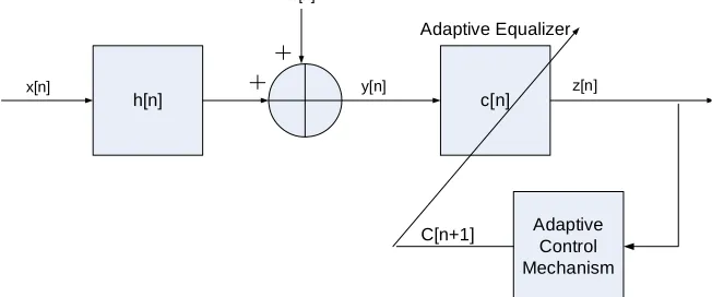
The system under consideration is illustrated in Figure 1, where we make the following assumptions:

1) The input sequence x n

 

belongs to a constella-

tion input with zero mean.

2) The unknown SISO system defined as h n

 

is a

possibly nonminimum phase linear time-invariant filter in which the transfer function has no zeros on the unit

circle.

3) The equalizer c n

 

is a tap-delay line.

4) The noise w n

 

is an additive Gaussian white

noise with zero mean and variance 2

   

w E w n w n

 _  _

  

where

 

 and E

 

 denote the conjugate and expec-tation operator on

 

 and on

 

 respectively.

Comments:

1) In the communication field, the popular constella- tion inputs, have the property of zero mean. Therefore, many cost functions (and those that are used in this paper) are based on the assumption having a source with zero mean.

2) An adaptive FIR equalizer can be used only if the transfer function of the channel (modeled with a FIR filter) has no zeros on the unit circle.

3) The zeros of the channels' transfer function may be outside the unit circle (nonminimum phase case). Thus, a cost function based on higher order statistics (HOS) is necessary for the equalization process. Second order sta- tistics (SOS) (auto-correlations or power spectra) based methods cannot be used if the channel is nonminimum phase since these methods are blind of the channel, whereas phase information is preserved in statistics of order higher than two. In this paper, we use HOS based cost functions.

4) There are many cases such as the wired case in which the channel is static, namely, does not change in time or almost does not change in time. Thus, the chan- nel may be described as a time-invariant filter. Since we model the channel as a time-invariant FIR filter, the channel coefficients will not vary with time.

5) Assumptions 1 - 4 were also made in many other papers dealing with the blind adaptive equalization prob- lem ([2,9,10] to name a few of them).

The sequence x n

 

is sent through the system h n

 

and is corrupted with noise w n

 

. Therefore, the equal- izer’s input sequence y n

 

may be written as:

       

y n x n h n w n (1)

where “*” denotes the convolution operation. The equal-

h[n] c[n]

w[n]

x[n] y[n] z[n]

Adaptive Equalizer

[image:2.595.135.461.581.717.2]

Adaptive Control Mechanism C[n+1]

ized output signal can be written as:

  



ej

   

z n x nD p n w n (2)

where D is a constant delay,  is a constant phase shift,

 

p n is the convolutional noise, namely, the residual

convolutive distortion arising from the difference be- tween the ideal equalizer’s coefficients and those chosen in the system and w n

 

   

c n



w n

 . Next we turn to the adaptation mechanism of the equalizer which is based on a predefined cost function F z n



 that character-

izes the convolutive distortion, see [4,9-12]. Minimizing this F z n

 

 with respect to the equalizer parameters

will reduce the convolutional error. Minimization is per- formed with the gradient descent algorithm that searches for an optimal filter tap setting by moving in the direc- tion of the negative gradient-cF z n

 

 over the sur-

face of the cost function in the equalizer filter tap space [13]. Thus the updated equation is given by [13]:



  



 



 

_{ }

 

 

1 _c

c n c n F z n F z n

c n y n

z n           _{ }         (3)

where  is the step-size parameter, c n

 

is the

equalizer vector where the input vector is

 





T

[ ] 1

y n _y n  y n N _ and N is the equal-izer's tap length. The operator denotes for trans-pose of the function

 

T

 

.

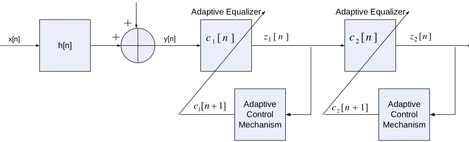
Next, we turn to describe our new proposed system (Figure 2) with two blind adaptive equalizers connected in series where the first and second blind adaptive equal-izer have N1 and N2 coefficients respectively. The input signal to the first blind adaptive equalizer is y n

 

(1).

The equalized output from this equalizer, given by

     

1

z n  y n c n₁ , is then sent to the input of the sec-

ond blind adaptive equalizer. Thus, the total equalized output signal may be written as:

 

         

2 1 2 1 2

z n z n c n y n c n c n (4)

The update equations for the first and second blind adaptive equalizer are given by:





 



 



 

_{ }

 

 

1

1 1 1 1

1

1 1

1

1 c

c n c n F z n F z n

c n y n

z n           _{ }         (5)





 



 



 

_{ }

 

 

2

2 2 2 2

2 1

2 2

2

1 c

c n c n F z n F z n

c n z n

z n           _{ }         (6)

where ₁ and ₂ are the step-size parameters. Ac- cording to [14], the more coefficients in the equalizer, the more “noise” is introduced into the adaptation of each coefficient by the simultaneous adaptation of the other coefficients. Thus, this might be the reason why having a larger convergence speed for higher numbers of coeffi- cients in the equalizer. It should be pointed out, that this was also observed in [15] where higher numbers of coef- ficients in the equalizer have lead to a longer conver- gence speed. Obviously, choosing a higher step-size pa- rameter may increase the convergence speed but on the same time it increases also the residual ISI which might not meet any more the system’s requirements. In order to get improved convergence speed, two blind adaptive equalizers connected in series, c n1

 

and c n2

 

, are

used where 1

 

is responsible for getting fast con-

vergence speed (achieved with N1 < N2 < N and 1

c n

 ) and ₂

 

compensates the high residual ISI left at the output from

c n

 

1 (accomplished by setting 2

c n  ).

We may express the two blind adaptive equalizers con- nected in series as an equivalent filter defined by

 

1

   

2 with N1 + N2− 1 filter taps. In our

proposed system, N = N1 + N2− 1 where N, N1 and N2 have odd values. In all our cases we have chosen N1 to be

c n c n c n

approximately half of N, 1 and 2 ₂

   . h[n] w[n] x[n] y[n] Adaptive Equalizer Adaptive Control Mechanism Adaptive Equalizer Adaptive Control Mechanism ] [ 1 n

z z₂[n]

] 1 [ 1 n

c _c2[n1]

] [ 1 n

[image:3.595.60.536.576.720.2]

c

c

2

[

n

]

3. Simulation

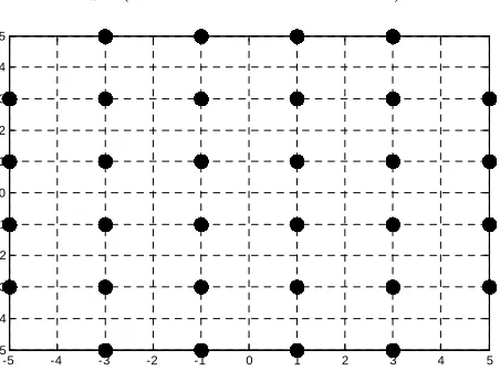
In this section we compare the equalization performance of our new proposed system with two blind adaptive equalizers connected in series with a system using only a single blind adaptive equalizer. For simplicity we used the digital communication case where the the source sig- nal belongs to a 16 QAM (Quadrature Amplitude Modu- lation-QAM) constellation (a modulation using ±{1, 3} levels for in-phase and quadrature components) and to a 32QAM input (Figure 3). But, in order to show that the new proposed method also works well for other source inputs and not only for those belonging to the digital communication case, we used a third source signal x n

 

where the real and imaginary parts of x n

 



were inde- pendently uniformly distributed within  4, 4



. The ISI is often used as a measure of performance in equalizer’s applications, defined by

 

2 2

max

2 max

m

s m s ISI

s

 





  

 (7)

where s_max is the component of s , given in (8),

having the maximal absolute value.

   

     

1 2

for system 1 for system 2 s c n h n

s c n c n h n

 

  



 (8)

where system 1 and system 2 are defined as the system with a single blind adaptive equalizer and the system with two blind adaptive equalizers connected in series respectively. In the following we define h n

 

as a

channel. Two different channels were considered.

Channel 1 (initial ISI = 0.88): The channel parameters were determined according to:



0.4851, 0.72765, 0.4851

n

h   





.

Channel 2 (initial ISI = 1.402): The channel parame- ters were determined according to [11]:



0.2258,0.5161,0.6452,0.5161

n

h  .

-5 -4 -3 -2 -1 0 1 2 3 4 5

[image:4.595.62.288.553.726.2]

-5 -4 -3 -2 -1 0 1 2 3 4 5

Figure 3. 32QAM constellation.

As it can be seen, the ISI caused by the chosen chan- nels is very high which means that the initial convolutive distortion level is very high. In our simulation, we used two different predefined cost functions F z n k

 



(where k0,1, 2 and z n₀

   

z n ) in order to show that the new proposed system is not a special case for a specific predefined cost function. Thus, for Godard’s method [4] we have:

 

 

 

 

 

 

4 2 2 k k k k

E x n F z n

z n z n

z n _{E x n}

      _{    } _  _  _  _       (9)

while for the WNEW algorithm [2] the function

 

 

k

k

F z n z n

 

  

 is defined by:

 

 



_



_

 

_{ }



_



_

 









 









 

3 2 3 2 Re Re Im Im k k k k k z n F z n

z n _{E x n}

z n

j z

E x n

     _{   }    _  _            _{ }    _{ }     n (10)

[image:5.595.59.285.79.273.2] [image:5.595.308.537.85.274.2]

Figure 4. Equalization performance comparison between the system with a single blind adaptive equalizer and the system with two blind adaptive equalizers connected in se-ries. In both cases we used a 16QAM source input going through channel 1 and the WNEW algorithm. The averaged results were obtained in 100 Monte Carlo trials for SNR = 10 dB. We set N = 11, N1 = 5, N2 = 7, μ = μ1 = 0.001 and μ2 = 0.0005.

Figure 5. Equalization performance comparison between the system with a single blind adaptive equalizer and the system with two blind adaptive equalizers connected in se-ries. In both cases we used a 16QAM source input going through channel 1 and the WNEW algorithm. The averaged results were obtained in 100 Monte Carlo trials for SNR = 30 dB. We set N = 11, N1 = 5, N2 = 7, μ = μ1 = 0.001 and μ2 = 0.0005.

[image:5.595.59.284.375.561.2]

When this occurs, the equalized output is driven to a DFE (decision feedback equalizer) for further equaliza- tion improvement. In our case (Figures 6 and 7), the eye diagram is considered as already open when the residual ISI is less than –15 [dB]. According to Figures 67 the residual ISI for both systems (1 and 2) is much lower

Figure 6. Equalization performance comparison between the system with a single blind adaptive equalizer and the system with two blind adaptive equalizers connected in se-ries. In both cases we used a 16QAM source input going through channel 2 and the WNEW algorithm. The averaged results were obtained in 100 Monte Carlo trials for SNR = 30 dB. We set N = 21, N1 = 9, N2 = 13, μ = μ1 = 0.0002 andμ2 = 0.0001.

Figure 7. Equalization performance comparison between the system with a single blind adaptive equalizer and the system with two blind adaptive equalizers connected in se-ries. In both cases we used a 16QAM source input going through channel 2 and the Godard algorithm. The averaged results were obtained in 100 Monte Carlo trials for SNR = 30 dB. We set N = 21, N1 = 9, N2 = 13, μ = μ1 = 0.00001 and

μ2 = 0.000005.

[image:5.595.309.537.376.561.2]

[image:6.595.59.285.84.277.2]

Figure 8. Equalization performance comparison between the system with a single blind adaptive equalizer and the system with two blind adaptive equalizers connected in se-ries. In both cases we used a source signal x[n] where the real and imaginary parts of x[n] were independently uni-formly distributed within [−4, +4]. For both cases, the source input was sent through channel 1 and the WNEW algorithm was used. The averaged results were obtained in 200 Monte Carlo trials for SNR = 10 dB. We set N = 11, N1 = 5, N2 = 7, μ = μ1 = 0.001 and μ2 = 0.0005.

[image:6.595.308.536.84.277.2] [image:6.595.310.537.380.583.2]

case) where the x and y-axis of the signal are dependent. Figure 9 shows the equalization performance of our new proposed system (system 2), namely the ISI as a function of iteration number for the 32QAM input case, channel 1 and SNR = 10 [dB], compared with system 1. According to Figure 9, the equalization performance improvement is seen in the residual ISI as well as in the convergence speed. According to simulation results we may say that the equalization performance improvement is obtained in the low SNR environment as well as in the case where the convergence speed of the deconvolution process of a single blind adaptive equalizer is very long.

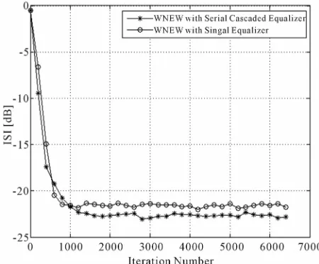
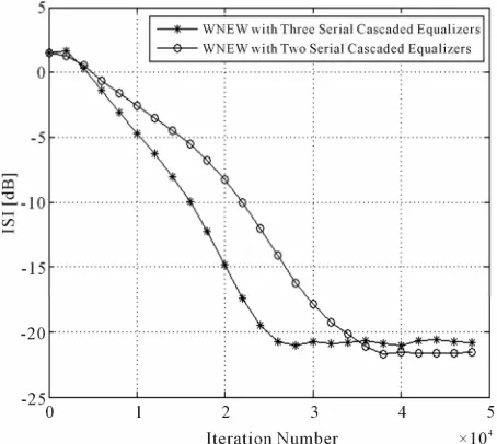
The simulation results for the two serial cascaded adaptive equalizers made us wonder whether it is possi- ble to get further equalization performance improvement by using three serial cascaded adaptive equalizers. Fig- ure 10 shows the equalization performance comparison, namely, the ISI as a function of iteration number between a system with two serial cascaded blind adaptive equal- izers and a system with three blind adaptive equalizers connected in series for the 16QAM source input, channel 2 and SNR = 30 [dB]. According to Figure 10, improved equalization performance is obtained from the conver- gence speed point of view with the three serial cascaded blind adaptive equalizers compared with the system with two blind adaptive equalizers connected in series. Next, we compare a system using two serial cascaded blind adaptive equalizers with a system using three blind adap-

Figure 9. Equalization performance comparison between the system with a single blind adaptive equalizer and the system with two blind adaptive equalizers connected in se-ries. In both cases we used a 32QAM source input going through channel 1 and the Godard algorithm. The averaged results were obtained in 100 Monte Carlo trials for SNR = 10 dB. We set N = 11, N1 = 5, N2 = 7, μ = μ1 = 0.00002 and μ2 = 0.00001.

Figure 10. Equalization performance comparison between the system with two serial cascaded blind adaptive equal-izer and the system with three blind adaptive equalequal-izers connected in series. In both cases we used a 16QAM source input going through channel 2 and the WNEW algorithm. The averaged results were obtained in 50 Monte Carlo tri-als for SNR = 30 dB. We set N1 = 9, N2 = 13, μ1 = 0.0002 and

μ2 = 0.0001 for the two serial cascaded equalizer, N1 = 3, N2 = 7, N3 = 13, μ1 = 0.0002,  

 

2

0.0002

2 0.0001333

 



μ and

3

0.0002

0.0000666

 



μ for the three serial cascaded eq-

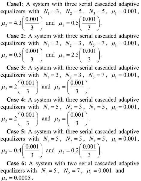
tive equalizers connected in series for the 16QAM source input, channel1 and SNR = 10 [dB]. Let us denote 6 cases:

Case1: A system with three serial cascaded adaptive equalizers with N13, N25, N35, 10.001,

2

0.001 4.3

3   _

 



 and 2

0.001 0.5

3   _ _

 .

Case 2: A system with three serial cascaded adaptive equalizers with N₁3, N₂3, N₃7, ₁0.001,

2

0.001 0.5

3   _

 



 and 2

0.001 2.5

3   _ _

 .

Case 3: A system with three serial cascaded adaptive equalizers with N13, N23, N37, 10.001,

2

0.001 2

3  _{ }

 



 and 2

0.001 3  _{ } _

 .

Case 4: A system with three serial cascaded adaptive equalizers with N₁5, N₂3, N₃5, ₁0.001,

2

0.001 2

3  _{ }

 



 and 2

0.001 3  _{ } _

 .

Case 5: A system with three serial cascaded adaptive equalizers with N15, N25, N35, 10.001,

2

0.001 0.4

3   _

 



 and 2

0.001 0.2

3   _ _

 .

Case 6: A system with two serial cascaded adaptive equalizers with N15, N27, 10.001 and

2 0.0005

[image:7.595.56.291.121.422.2] [image:7.595.59.285.470.657.2]

  .

Figure 11 shows the equalization performance com- parison, namely, the ISI as a function of iteration number between the system with two serial cascaded blind adap-

Figure 11. Equalization performance comparison between the system with two serial cascaded blind adaptive equal-izer and several systems with three blind adaptive equaliz-ers connected in series. In all cases we used a 16QAM source input going through channel 1 and the WNEW algo-rithm. The averaged results were obtained in 100 Monte Carlo trials for SNR = 10 dB.

tive equalizers named as Case 6 and a system with three blind adaptive equalizers connected in series (with five different cases named as Cases 1-5) for the 16QAM source input, channel 1 and SNR = 10 [dB]. According to

Figure 11, the best equalization performance is obtained for Case 6. In other words, for channel 1, SNR = 10 [dB] and 16QAM source input, the best equalization perfor- mance is obtained with two serial cascaded blind adap- tive equalizers and not with a system using three blind adaptive equalizers connected in series.

4. Conclusion

In this paper, we have shown another promising ap- proach for accelerating the convergence speed of a blind adaptive equalizer with N1 + N2− 1 coefficients (where N1 and N2 are odd values) that does not use the variable step-size parameter approach and that is applicable not only for the CMA or MCMA algorithm. We have shown that a system with two blind adaptive equalizers con- nected in series where the first and second blind adaptive equalizer have N1 and N2 (N1 < N2) coefficients respec- tively achieves improved equalization performance compared with the case where a single blind adaptive equalizer is applied with N1 + N2 − 1 coefficients. It should be pointed out that the same algorithm (cost func- tion) was used for updating the filter taps for the different equalizers. Thus, the equalization performance im- provement of the blind adaptive equalizer was not achieved due to a better cost function. The equalization performance improvement was mainly seen in the con- vergence speed which was found to be approximately faster by a factor of two for the low SNR environment as well as in the case where the convergence speed of the deconvolution process of a single blind adaptive equal- izer is very long. Since the new approach used fixed step-size parameters, it might be possible that further equalization performance improvement may be obtained if instead for the fixed step-size parameter we use the variable step-size parameter approach. But, this is be- yond this paper.

5. Acknowledgements

I would like to thank the anonymous reviewers for their helpful comments.

REFERENCES

[1] C. Feng and C. Chi, “Performance of Cumulant Based Inverse Filters for Blind Deconvolution,” IEEE Transac- tion on Signal Processing, Vol. 47, No. 7, 1999, pp.

1922-1936. doi:10.1109/78.771041

[2] M. Pinchas and B. Z. Bobrovsky, “A Maximum Entropy Approach for Blind Deconvolution,” Signal Processing

doi:10.1016/j.sigpro.2005.12.009

[3] C. L. Nikias and A. P. Petropulu, “Higher-Order Spectra Analysis a Nonlinear Signal Processing Framework,” Chapter 9, Prentice-Hall, Upper Saddle River, 1993, pp. 419-425.

[4] D. N. Godard, “Self Recovering Equalization and Carrier Tracking in Two-Dimenional Data Communication Sys-tem,” IEEE Transactions on Commications, Vol. 28, No.

11, 1980, pp. 1867-1875. doi:10.1109/TCOM.1980.1094608

[5] M. A. Demir and A. Ozen, “A Novel Variable Step Size Adjustment Method Based on Autocorrelation of Error Signal for the Constant Modulus Blind Equalization Al- gorithm,” Radioengineering, Vol. 21, No. 1, 2012, pp.

37-45.

[6] R. Hamzehyan, R. Dianat and N. C. Shirazi, “New Vari- able Step-Size Blind Equalization Based on Modified Constant Modulus Algorithm,” International Journal of Machine Learning and Computing, Vol. 2, No. 1, 2012,

pp. 30-34.

[7] X. Zhang, L. S. Li, D. F. Zhuo and Z. S. Dong, “A New Adaptive Step-Size Blind Equalization Based on Auto-correlation of Error Signal,” 7th International Con- fer-ence on Signal Processing, Beijing, 31 August-4

Sep-tember 2004, pp. 1719-1722.

[8] L. Y. Zhang, L. Chen and Y. S. Sun, “Variable Step-Size CMA Blind Equalization Based on Non-Linear Function of Error Signal,” International Conference on Communi-cations and Mobile Computing, Kunming, 6-8 January

2009, pp. 396-399.

[9] M. Lazaro, I. Santamaria, D. Erdogmus, K. E. Hild, C. Pantaleon and J. C. Principe, “Stochastic Blind Equaliza-tion Based on pdf Fitting Using Parzen Estimator,” IEEE Trans. on Signal Processing, Vol. 53, No. 2, 2005, pp. 696-704. doi:10.1109/TSP.2004.840767

[10] O. Shalvi and E. Weinstein, “New Criteria for Blind De-convolution of Nonminimum Phase Systems (Channels),”

IEEE Transactions on Information Theory, Vol. 36, No.

2, 1990, pp. 312-321. doi:10.1109/18.52478

[11] M. Pinchas, “A MSE Optimized Polynomial Equalizer for 16QAM and 64QAM Constellation,” Signal, Image and Video Processing, Vol. 5, No. 1, 2011, pp. 29-37. doi:10.1007/s11760-009-0138-z

[12] G.-H. Im, C. J. Park and H. C. Won, “A Blind Equaliza-tion with the Sign Algorithm for Broadband Access,”

IEEE Communication Letters, Vol. 5, No. 2, 2001, pp.

70-72. doi:10.1109/4234.905939

[13] A. K. Nandi, “Blind Estimation Using Higher-Order Sta-tistics,” Chapter 2, Kluwer Academic, Boston, 1999, pp. 78-79.

[14] E. A. Lee and D. G. Messerschmitt, “Adaptive Equaliza-tion,” In: E. A. Lee and D. G. Messerschmitt, Eds., Digi-tal Communication, 2nd Edition, Kluwer Academic

Pub-lisher, Boston, 1997.