Happiness, Dynamics and Adaptation

Munich Personal RePEc Archive

Happiness, Dynamics and Adaptation

Piper, Alan T.

Universität Flensburg

December 2013

HAPPINESS, DYNAMICS AND ADAPTATION

Alan T. Piper*, **

Universität Flensburg

Internationales Institut für Management und ökonomische Bildung

Munketoft 3B, 24937 Flensburg, Deutschland

December 2013

ABSTRACT: This investigation employs dynamic panel analysis to provide new insights into the phenomenon of adaptation. Using the British Household Panel Survey, it is demonstrated that happiness is largely (but not wholly) contemporaneous. This can help provide explanations for previous findings, where many events entered into in the past are often adapted to (like marriage and divorce), and others are not adapted to (like unemployment and poverty). An event – no matter when entered into - must have a contemporaneous impact on either the life of an individual or an individual’s perception of their life (or both) for it to be reflected in self-reported life satisfaction scores. This contemporaneous finding also explains other results in the literature about the well-being legacy of events.

*Email address for correspondence: [email protected]

2

Happiness, Dynamics and Adaptation

When we have an experience . . . on successive occasions, we quickly begin to adapt to it, and the experience yields less pleasure each time... Psychologists calls this habituation, economists call it declining marginal utility, and the rest of us call it marriage (Gilbert 2006, p.144).

1. Introduction

The economic analysis of well-being has provided evidence that, in terms of happiness,

individuals get used to, or adapt to, some events and not to others, but has not yet offered an

explanation why some events are adapted to and others are not. Previous research (references

at the end of this paragraph) suggests that events that are adapted to include marriage,

divorce, widowhood, having a child, and exogenous income boosts like winning a lottery,

whereas the events that are not adapted to (or not fully adapted to) include unemployment,

disability and poverty. This has been demonstrated largely with panel data from Britain and

Germany, and to a lesser extent Australian and Korean data, often with static fixed effects

estimation methods utilising dummy variables to represent years after the event (as well as, in

some cases, dummy variables for lead or anticipation effects). Some prominent examples are

as follows: Lucas et al. 2004; Lucas 2005; Gardener and Oswald 2006; Stutzer and Frey

2006; Clark et al. 2008a; Oswald and Powdthavee 2008; Frijters et al. 2011; Rudolph and

Kang 2011; Clark et al. 2013; Clark and Georgellis 2013.

The contribution of this investigation is to provide a general explanation of why individuals

adapt to some things and not others. To do so, this study employs a relatively new method for

the economic analysis of the concept of happiness: dynamic panel analysis utilising General

Method of Moments (GMM) estimation. Other well-being studies that use this model

include: Powdthavee 2009; Della Giusta et al. 2010; Bottan and Perez-Truglia 2011; Piper

2012; Wunder 2012. Because dynamics are explicitly modelled, insights are provided for the

analysis of adaptation. The ‘workhorse’ model for the investigation of adaptation, like the

3 advantage of the rich nature of nationally representative samples, like the British Household

Panel Survey (BHPS) and the German Socio-Economic Panel (SOEP). Such an analysis has

provided many insights for a scientific understanding of well-being. Useful reviews of these

studies include Dolan et al. (2008), Clark et al. (2008b) and MacKerron (2012). This study

demonstrates that fixed effects analyses neglect to consider the possibility of omitted

dynamics in such estimations. The presence or otherwise of serial correlation is rarely (if

ever) tested for in the literature, and the analysis here, using a well-known and well-utilised

data set, demonstrates that this is a substantial issue: the presence of serial correlation in the

idiosyncratic error term means that there are omitted dynamics in the FE estimates. As King

and Roberts (2012) forcefully argue, this should not be treated as a problem to be fixed by

adjusting the standard error but instead as an opportunity to take advantage of this

information and respecify the model.

The respecification presented here, which results from the strongly significant finding of

serial correlation in the idiosyncratic error term, is to employ dynamic panel methods. In

practice, this introduces a lagged dependent variable on the right-hand-side of the equation,

which substantially changes the interpretation of the coefficients for the independent

variables. Such an analysis also introduces more methodological considerations, including the

ability to choose whether the independent variables are endogenous and exogenous. Such a

choice can substantially change the significance of any association between well-being and

some important independent variables. A further advantage of dynamic panel methods over

standard fixed effects analysis is the ability to distinguish between long-run effects and

contemporaneous effect of various variables on happiness. The results directly obtained from

such an analysis are the new information or contemporaneous effects, and a quick

post-estimation calculation can provide the long-run coefficients. Such models are more complex

4 necessary diagnostic tests. A weakness of the majority of the existing studies that make use of

dynamic panel models in a well-being context is that they either appear to misunderstand or

do not discuss the key diagnostics. By discussing these and highlighting these diagnostic

related concerns regarding other studies, this investigation also aims to help future well-being

research.

This paper is organised as follows. Section 2 discusses the data used, presents results from

fixed effects analysis, and demonstrates that the fixed effects analysis contains serial

correlation, an indicator of omitted dynamics. Section 3 discusses a solution to the problem of

omitted dynamics: dynamic panel analysis. As mentioned above, such a method adds

complexity to the standard fixed effects analysis and its key advantages and issues are more

fully explained in section 3. Using the same data employed in section 2, Section 4 presents

and discusses the results from the dynamic panel analysis. Section 5 discusses the

implications of using dynamic panel analysis, and these particular results, for the on-going

adaptation discussion. Section 6 concludes.

2. The Economics of Happiness: static panel analysis

This section briefly discusses the data, and the choice of a particular static panel model.

Subsequently, the results are presented from the preferred static panel model, before

explaining why dynamic panel analysis is often necessary. The data come from the British

Household Panel Survey (BHPS), a widely used data set within the economics of happiness

literature, with the dependent variable being life satisfaction, measured on an ordinal scale

from 1 to 7, ‘not at all satisfied’ to ‘completely satisfied’.1

The chosen independent variables,

common to most previous studies, are income, job status, marital status, education, and

1

5 health. Wave and regional dummies are also included in the estimates.2 The other variables in

the regression account for age bands.

Initial diagnostic tests (not reported here) establish that the workhorse model, FE, is the

preferred static model, being more appropriate than RE and OLS. This finding is typical in

the literature and somewhat expected: the benefits of panel analysis as compared to pooled

cross section analysis are numerous. Arguably, the most important benefit is that individual

heterogeneity can be controlled for, and this helps us overcome Bentham’s well-known

apples and oranges concern. Fixed effects estimations investigate variation within an

individual, which removes the need to compare between individuals. This estimation method

effectively ‘controls’ for the time invariant characteristics of each individual, meaning that

FE regressions allow (or control) for differences in personality and disposition that may be

important determinants of life satisfaction.

The specification adopted here is typical of the estimations in the empirical economic

literature, and is as follows:

Where LSit _{is the response of individual i at time t to the life satisfaction question.}

χ

i is a 1 x

k vector of covariates and

β

specific residual (the individual fixed effect) and is the ‘usual’ residual. Results for these

regressions are presented in table 1.

[TABLE ONE ABOUT HERE]

2

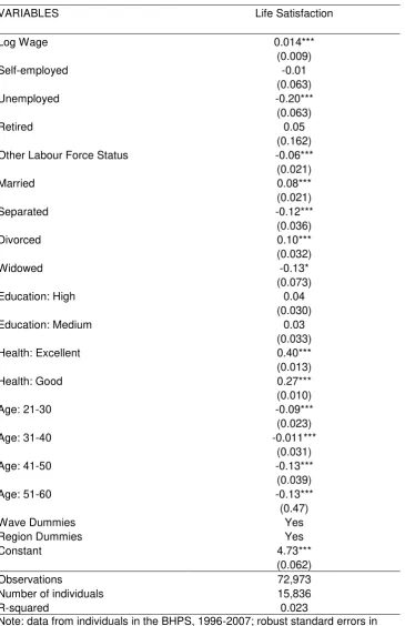
6 The results in table 1 are similar to results of previous studies. The following are positive and

statistically significant for life satisfaction: log real wage; being married; being divorced3 and

categorising health as good or excellent. Being unemployed, having a labour force status

classed as other4, being separated or widowed, are all statistically significant and negative for

life satisfaction. Not shown, but by gender separately the results are similar with two

exceptions: for males education is positive and statistically significant with life satisfaction,

while for females unemployment is only significant at a 90% confidence level (with a p-value

of around 0.06). Furthermore, for both genders separately and together, the coefficients on

the age range dummy variables are in line with the familiar U-shape relationship of age with

life satisfaction found in the wider literature. However, analysis does not (and should not) end

here with static analysis.

Wooldridge’s (2002) test for serial correlation in the idiosyncratic error term in panel data,

implemented in Stata by the user-written xtserial command (Drukker 2003), rejects the null

hypothesis of no first order autocorrelation with a p-value of 0.000. (i.e., in practical terms,

the null can be rejected with certainty).5This is potentially useful information, and it is clear

that such a firm rejection of the assumption of no autocorrelation needs, somehow, to be

modelled. One possibility is to recognise the clusters involved in the panel regression and to

correct the standard errors accordingly. However, this treats the omitted dynamics detected

by the diagnostic test as a problem rather than an invitation to respecify the model to include

3

Using the same dataset as the analysis here, the BHPS, Clark and Georgellis (2013), via a static panel analysis using lead and lag dummy variables, demonstrate that, on average, the newly divorced receive a boost to their happiness that they eventually adapt to.

4

This might be caring for someone, on maternity leave, a student, on a government training scheme, a family carer, long-term sick, disabled or one of a handful of people in the dataset who fit none of the possible categories.

5

7 the omitted dynamics in the estimated part of the model, thus exploiting this additional

information in estimation. This argument has recently been strongly supported by King and

Roberts (2012) in a study of robust standard errors:

Robust standard errors now seem to be viewed as a way to inoculate oneself from criticism. We show, to the contrary, that their presence is a bright red flag, meaning “my model is misspecified”… it appears to be the case that a very large fraction of the articles published across fields is based on misspecified models. For every one of these articles, at least some quantity that could be estimated is biased (p. 2).6

Accordingly, a potentially more interesting solution is to estimate a dynamic panel model.

3. The Economics of Happiness: dynamic panel analysis discussion

This section is informed by finding the presence of first order serial correlation in the

idiosyncratic error term in the static estimation of section 2. Such a result can mean that the

estimates generated by static panel analysis are inefficient and potentially misspecified.

Adding dynamics to the model is usually undertaken by including a lag of the dependent

variable as a right hand side variable. Hence, what is estimated is the following standard

equation (with the independent variables excluded for clarity):

As this is a panel model each observation is indexed over i (= 1…N) cross-section groups

(here individuals) and t (= 1…T) time periods (here, annual observations). Equation 2 is a

first-order dynamic panel model, because the explanatory variables on the right-hand side

include the first lag of the dependent variable (yi, t-1). The composed error term in parentheses

combines an individual-specific random effect to control for all unobservable effects on the

dependent variable that are unique to the individual and do not vary over time (i), which

6_{“We strongly echo what the best}

8 captures specific ignorance about individual i, and an error that varies over both individuals

and time (_it), which captures our general ignorance of the determinates of yit. However, this

cannot be estimated accurately by OLS or by fixed effects estimation. An OLS estimator of

 in equation 2 is inconsistent, because the explanatory variable y_i,t1 is positively

correlated with the error term due to the presence of individual effects. A fixed effects

estimation does not have this inconsistency because the equation is transformed to remove

the individual effect, as in equation 3.

However, equation (3) exhibits a different problem of correlation between the transformed

lagged dependent variable and transformed error term. Here the overall impact of the

correlations is negative, and is the well-known Nickell (1981) bias. Bond (2002) states that

these biases can be used to provide an informal test for an estimator of the lagged dependent

variable: the estimated coefficient should be bounded below by the outcome from OLS

(which gives the maximum upwards bias) but above by the fixed effects estimate (which

gives the maximum downwards bias).7

Due to these problems, the standard approach is to find a suitable instrument that is correlated

with the potentially endogenous variable (the more strongly correlated the better), but

uncorrelated with εit. Because instrumentation is not confined to one instrument per

parameter to be estimated, the possibility exists of defining more than one moment condition

per parameter to be estimated. It is this possibility that is exploited in the General Method of

Moments (GMM) estimation of dynamic panel models, first proposed by Holtz-Eakin et al.

7

This bias has been misunderstood in some of the well-being work which estimates similar equations. Della

Giusta et al (2010) states that the biases are general, and “therefore, we have reported both of the [whole of]

OLS and fixed effects results as a comparison (both of which do not include a lagged dependent variable)”

9 (1988).8 The two models popularly implemented are the “difference” GMM estimator (Arellano and Bond, 1991) and the “system” GMM estimator (Arellano and Bover 1995).

Greene (2002, p.308) explains that suitable instruments fulfilling the criteria mentioned

above come from within the dataset: the lagged difference (yit-2 – yit-3) ;and the lagged level y

it-2. Both of these should satisfy the two conditions for valid instruments, since they are likely

to be highly correlated with (y_i,t1 y_i,t2) but not with





of such “internal” instruments (i.e., from within the dataset) that the GMM estimators exploit.

The “difference” GMM estimator follows the Arellano and Bond (1991) data transformation,

where differences are instrumented by levels. The “system” GMM estimator adds to this one

extra layer of instrumentation where the original levels are instrumented with differences

(Arellano and Bover 1995).

These estimators, unlike OLS and conventional FE and RE estimation, do not require

distributional assumptions, like normality, and can allow for heteroscedasticity of unknown

form (Verbeek, 2000, pp. 143 and 331; Greene, 2002, pp.201, 525 and 523). A more

extensive discussion of these methods is beyond the scope of this investigation, but the

references provided above and papers by Roodman (e.g. 2006, 2007, and 2009) are very

informative.9 Powdathee (2009) in a study that is wonderfully titled and quotes the singer

Barry Manilow, investigates marriage and well-being using GMM estimation, arguing that

this can also solve the problem of measurement error bias with self-reported life satisfaction.

A further advantage of GMM estimation and the use of “internal” instruments is that applied

researchers can select which regressors are potentially endogenous and which exogenous

with respect to life satisfaction. A key choice with GMM panel analysis, and the discussion

8

GMM was developed by Lars Peter Hansen, work that led, in part, to him being selected as one of the Nobel Prize winners for Economics in 2013. See Hansen (1982) for more information on the General Method of Moments,or Hall (2005) for a detailed textbook treatment.

9

10 below will show how important this decision is. Similarly, the discussion below will focus on

the diagnostic tests and the interpretation of the results in some detail because other studies

that use this method (in the context of a dynamic panel analysis of happiness) do not discuss

them, partially discuss them, or appear to misunderstand them. Furthermore, this is also

discussed in some detail because the method employed is relatively new in the well-being

literature, and somewhat more complex than the methods more commonly used therein.

Thus, before estimating any dynamic panel model there are two important (and linked)

considerations. Firstly, are the regressors potentially endogenous or strictly exogenous?

Secondly, how many instruments to use? With happiness equations many of the regressors

are potentially endogenous – does marriage, for example, make someone happy or are happy

people more likely to get married (or are both determined by underlying but omitted

variables) – and the choice of endogeneity or exogeneity can influence the coefficients

subsequently estimated. Diagnostics are available and built in with xtabond2, the Stata

command employed for empirical analysis, to help with this choice.

The choice of which regressors are to be treated as endogenous and exogenous is also bound

up with the consideration of how many instruments should be used, because that choice

generates the instruments. More regressors treated as endogenous means more instruments

are employed, ceteris paribus. Researchers can also affect the instrument count by changing

the lag length to be used for instrumentation, and good practice is to test results for their

robustness to different lag length choices (and hence different instrument counts). Diagnostic

tests are available for the appropriateness of the instrumentation collectively, and the subsets

of instruments created by the regressors that are treated as exogenous or endogenous, as well

11 instruments can be tested should the researcher want to.) These tests are asking whether the

instruments are exogenous to the error term, and are returned to below.

Additionally, xtabond2 contains a built in check on first and second order autocorrelation in

first differences, which is an additional check on the appropriateness of the instrumentation.10

For this investigation, the “system” GMM estimation was undertaken twice, with the

difference being gender. The reason is largely pragmatic: such estimations are

computationally intensive and it was not possible to perform the estimate for the whole

sample.11 In both cases, the diagnostics of the chosen models indicate that first order

autocorrelation is present, but second order is not (as shown in table 2). This is expected (and

necessary): the difference of lags and the difference of levels are correlated (first order),

However, the second differences are not and thus are valid for instrumentation.12

The serial correlation diagnostics in the above paragraph reflect the outcome of the chosen

model for each gender, a decision that was made after testing many variants regarding lag

lengths, instrumentation, and the choice regarding the endogeneity or exogeneity of

regressors. These choices matter. They matter for the coefficients of the independent

variables (but not really for the lagged dependent variable for which the coefficient which

was fairly stable in all of the estimates), and the necessary exogneiety of the instruments.

Unsurprisingly, with the models ultimately chosen, the various tests of the instruments

indicate that they are suitable in each case – the null hypothesis of exogenous instruments

10

Recall the explanation presented above utilising Greene (2002).

11

Every dynamic regression both shown here, and undertaken as part of the diagnostic testing, employed the twostep robust procedure that utilises the Windmeijer (2005) finite sample correction for the two-step covariance matrix. Without this, standard errors have been demonstrated to be biased downwards (Windmeijer 2005).

12

12 (what we want) cannot be rejected. The Hansen (1982) test J statistic13 of all overidentifying

restrictions, with a p-value of approximately 0.76 (for males) and 0.60 for females, does not

reject the null of instrument validity indicating at least a sixty percent chance of a type one

error if the null is rejected. This is higher than Roodman’s recommended threshold of a p

-value of 0.25 where he (2007, p.10) warns that researchers

should not view a value above a conventional significance level of 0.05 of 0.10 with complacency. Even leaving aside the potential weakness of the test, those thresholds are conservative when trying to decide on the significance of a coefficient estimate, but they are liberal when trying to rule out correlation between instruments and the error term. A p value as high as, say, 0.25 should be viewed with concern. Taken at face value, it means that if the specification is valid, the odds are less than 1 in 4 that one would observe a J statistic so large.

The J tests, Hansen and Sargan, inspect all of the generated instruments together, with a null

of exogenous instruments. Low p-values mean that the instruments are not exogenous and

thus do not satisfy the orthogonality conditions for their use. Within the well-being area,

some of the GMM studies do not test (or at least report) the Hansen J test result, risking what

Sargan calls, more generally, a ‘pious fraud’. (Godfrey 1991, p.145). Other well-being studies

report a very low p-value and incorrectly assume that this indicates that the instruments are

appropriate for estimation.14

Valuable, but perhaps even more neglected, are the difference-in-Hansen (or C) tests. These

are diagnostic tests that inspect the exogeneity of a particular subset of instruments, and are

reported by xtabond2.15 This means that researchers can test their choice (and alternative

13

This has the advantage over the SarganJ test because it works in the presence of heteroscedasticity. Indeed, if the errors are believed to be homoscedastic then the Hansen test is the same as the Sargan test.

14

Bottan and Perez-Truglia (2011), for example, report p-values of <0.001 (Table 1A) and incorrectly state that

they cannot “reject the null of the Sargan test at the 1% level” (p.230). In this study, only once is the p-value of the Sargan test above 0.25. However, this may not necessarily invalidate all of its results because, for the reason put forward in footnote 11, the Hansen test (unreported) is the appropriate J test. Powdthavee (2009) reports the Hansen version of the J test, but the p-values are often under 0.25. In that article there is a supporting claim that

values between 0.1 and 0.25 are within Roodman’s (2007) acceptable range: as we can see from the Roodman

quote just above this is an incorrect claim.

15

13 choices) of which regressors should be treated as exogenous and which endogenous. This is

crucial since it can affect the overall J test result, and the choice considerably alters the

coefficients obtained for the independent variables (although not the lagged dependent

variable). This is discussed more in the results section with reference to other studies and is

well explained in Baum et al. (2003, sections 4.2 and 4.4) as well as the Roodman papers

referred to elsewhere. Here, such testing led to the treatment of marital status and health as

potentially endogenous for males, marital status, health, labour force status, and education for

females.16

The difference-in-Hansen tests also inspect the ‘initial conditions’ problem, which refers to

the relationship between the unobserved fixed effects and the observables at the time of the

start of the panel subset employed. For estimation to be valid, it is necessary that changes in

the instrumenting variables are uncorrelated with the individual-specific part of the error

term. This is tested by the difference-in-Hansen GMM test for levels, reported by xtabond2.

Roodman (2009, section 4) discusses this, and in the conclusion to the same article offers

advice regarding what diagnostic tests should be given along with the results: “several

practices ought to become standard in using difference and system GMM. Researchers should report

the number of instruments generated for their regressions. In system GMM, difference-in-Hansen

tests for the full set of instruments for the levels equation, as well as the subset based on the

dependent variable, should be reported” (Roodman 2009, p.156).

As recommended these are presented in the results table of the next section, where there is

also a discussion regarding how the coefficients should be interpreted. The introduction of the

lagged dependent variable means that the interpretation of the coefficients is somewhat

16

14 different from more conventional static fixed effects analysis. An understanding of the

interpretation of the coefficients, and particularly the coefficient on the lagged dependent

variable, is important generally, and for the discussion of adaptation in Section 5.

4. The Economics of Happiness: dynamic panel analysis results

This section presents and discusses the results from dynamic panel estimation, after an

explanation of how the coefficients need to be interpreted. A footnote above states that

coefficients obtained via OLS or FE were different from those obtained by dynamic panel

methods and could not directly be compared. As Greene asserts

Adding dynamics to a model … creates a major change in the interpretation of the equation. Without the lagged variable, the “independent variables” represent the full set of information that produce observed outcome yit. With the lagged variable, we

now have in the equation the entire history of the right-hand-side variables, so that any measured influence is conditional on this history; in this case, any impact of (the independent variables) xit represents the effect of new information. (2008, p.468,

emphasis added).

Thus, in a dynamic panel model, the independent variables only reflect new or

contemporaneous information conditional both on the other controls and the lagged

dependent variable, which itself represents the history of the model. This means that

contemporaneous associations of variables with life satisfaction can be usefully assessed via

dynamic panel methods, whereas anything historic (e.g. typically education) is captured in

the ‘black box’ of the lagged dependent variable itself.17

As a consequence of the lagged dependent variable being estimated (and the internal

instruments used), the number of observations will shrink somewhat because two consecutive

years are needed. In 2001, i.e. wave 11 of the BHPS, the life satisfaction question was not

15 asked which will mean two years of no data due to the missing lags. Given the necessity of (a

minimum of) two consecutive years, the number of observations from dynamic estimates will

be smaller than the observations used in the static analysis of section 2.

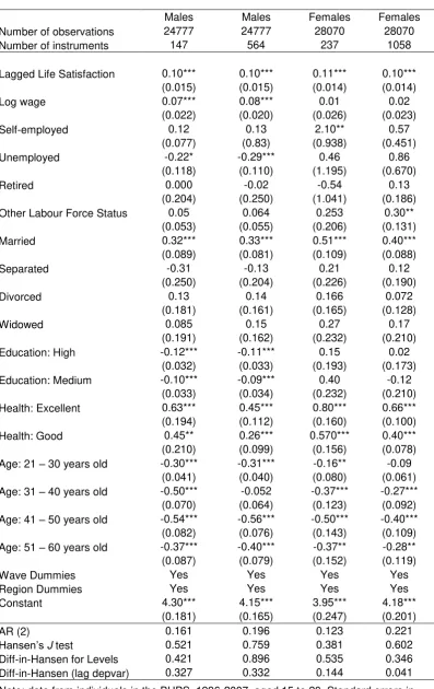
Table 2 displays the results for four estimations, two of which are for males and two for

females. The difference in the two columns for each gender is in the number of instruments

generated to obtain the coefficients. The estimation with the higher number of instruments

(for each gender) makes use of default instrumentation, which utilises the full length of the

sample to create instruments. In the other estimations for each gender, the lag length used is

restricted to the first available. The robustness (or otherwise) of the results to different

instrumentation will be discussed just after the discussion about the independent variable

coefficients.

[TABLE TWO ABOUT HERE]

For males, positive and statistically significant for life satisfaction are log wage, marriage,

health (both self-reported as good or excellent relative to a dummy variable capturing fair

health and worse responses); negative and statistically significant for life satisfaction are

unemployment and medium and high levels of education, assessed by qualifications obtained.

The coefficients on the age dummy variables are in line with the well-known U shape. These

results are robust to the number of instruments used being, for most variables, qualitatively

the same. In both male cases, the diagnostic tests are all supportive of the estimation choices

made. For females, the results are similar. The major exception is unemployment: the new

information coefficient (controlling for the history of the model) is insignificant. Recall that

the coefficient obtained by static fixed effects estimation was significant only at the 10%

16 some change based on the choice regarding the length of lags for instrumentation. The

diagnostic tests indicate which results we should lean towards being more accepting of.

Based on the AR(2) in first differences test and the Hansen J test the diagnostics, which are

now turned to, are acceptable and supportive of the estimation choices. However, this hides

the problem found by the difference-in-Hansen test for the instruments created by the lagged

dependent variable. The diagnostic problems for GMM estimation regarding females in the

BHPS are also found by Della Giusta et al (2010), where the null of having exogenous

instruments overall (i.e. Hansen J test) is comfortably rejected. This was often the case in

many of the estimations undertaken for this investigation, and this work here suggests that a

change in their choice of which regressors to treat as exogenous and endogenous would lead

to a more favourable Hansen J test result, leading to the non-rejection of the null of

exogenous instruments overall.18 The results presented are the best diagnostic outcomes for

the various possible choices regarding the endogeneity and exogeneity of the regressors and

yet there are still diagnostic problems. Based on the diagnostics, the preferred female model

is the one with lower instrumentation, be we must still be cautious about the results obtained

for females.

The lagged dependent variable is interesting, and informs the discussion regarding adaptation

of the next section. Here, we note that it is small, positive, statistically significant, and

consistent across the estimations (and indeed the estimations that formed part of the testing

for the results ultimately presented). To conclude this section, it is worth noting that in all

cases, dynamic GMM estimation for life satisfaction also passes Bond’s (2002) informal test

18

17 for a good estimator (mentioned above): the coefficient of 0.1 is lower than that obtained by

OLS (which is biased upwards) and higher than that obtained by fixed effects (which is

biased downwards).

5. Adaptation implications and discussion

The coefficient on lagged happiness in these dynamic estimations is itself interesting and, as

Greene informs us (see the quote that introduces the results section), this coefficient

represents the ‘entire history of the model’ i.e. the history of the process that generates

current levels of happiness. A little algebra expanding the lagged dependent variable

demonstrates this. In equation (4) is the life satisfaction of individual i in year t, is

an independent variable and is the usual error term. Starting with our simplified

specification in equation (4), we repeatedly substitute for the lagged dependent variable.

Substitute for in (4):

Substitute (5) into (4)

( )

Substitute for in (4):

Substitute (7) into (6)

( +

18 Going back further than four lags introduces more past values and more idiosyncratic error

terms too. By repeated substitution, it can be demonstrated that through the lagged dependent

variable dynamic specifications contain the entire history of the independent variable(s).

Thus, the lagged dependent variable tells us the influence of the past. In section 4 (and

elsewhere, as discussed below) this coefficient is positive, suggesting a persistence or inertia

effect from previous happiness: lagged happiness being positively associated with current

happiness. That the coefficient is small (around 0.1) means that the influence of the past is

minor, demonstrating that what are most important for the determination of current happiness

are current circumstances and events. To a greater or lesser degree, every study mentioned

previously that uses GMM for dynamic estimation finds a small, positive coefficient

(Powdthavee 2009; Bottan and Perez-Truglia 2010; Della Giusta et al 2010; Wunder 2012).

19

,20 Piper (2012) has also found a very similar coefficient for lagged life satisfaction for the

twenties age range, fifties age range, and when using the Caseness and Likert General Health

Questionnaire composites as a proxy for life satisfaction. These similar results for the lagged

dependent variable are obtained despite many differences including: in the equation

estimated; the datasets employed; alternate choices of exogneneity and endogeneity; and the

use of lags for other independent variables.

19_{Although, as mentioned earlier, many of these studies either don’}

t fully consider diagnostic tests or have results with inappropriate diagnostic test results my analysis suggests that altering the instrumentation choices has a substantial impact on the coefficients for the independent variables but only a small impact on the lagged dependent variable. In my regressions, testing the differing choices of endogeneity and exogeneity, the coefficient was almost always between 0.09 and 0.12. This means that studies where the independent variable coefficents are crucial (like Powdthavee 2009 and Della Giusta et al 2010) should be extra diligent with respect to the modelling choices discussed earlier.

20

Powdthavee (2009) does not consistently find a significant effect of lagged life satisfaction, however as mentioned previously the estimations do not exhibit good diagnostic test results. In the estimations that are closest to those of this investigation, (columns 7 and 8 of Table 2) he finds a small, positive significant effect of past life satisfaction of current life satisfaction. Wunder obtains almost exactly the same coefficient as those obtained in section 4 in regressions that do not employ the additional lags of the dependent variable. This is not reported in Wunder (2011) because it is not diagnostically appropriate, there is AR(2) serial correlation in the such estimates with the GSOEP. (Email correspondence). I have also found figures around 0.1 to 0.12 for

various estimations using the GSOEP too, but like Wunder’s work the diagnostics do not sufficiently support

19 Below, it is argued that this result is entirely consistent with current work on adaptation,

however in the literature another possible hypothesis and expectation has been put forward

for the coefficient on lagged happiness. Bottan and Perez-Truglia (2011) assert that past

happiness should be negatively correlated with current happiness (i.e. they expect negative

coefficient on lagged life satisfaction) supporting their notion of what they call general

habituation (in contrast to specific habituation which is getting used to a single event like, for

example, marriage or a pay rise). Because specific habituation occurs, they argue that general

habituation should occur: we adapt to marriage and divorce so perhaps we adapt to happiness

overall (an argument that ignores events like unemployment, to which people do not appear

to adapt (as in, for example, Clark et al. 2008a)). Bottan and Perez-Truglia (2011, p.224)

argue for general adaptation in their opening paragraph with this rationale (the oft-found

adaptation in the literature to specific incidents means that there is a general adaptation effect

too). In a later version of this paper, in support of general adaptation they refer to “what we

might recognise as the evolutionary origins of hedonic adaptation. The basic intuition is that

positive and negative hedonic states are costly from a fitness perspective: e.g. generating

feelings is a waste of energy for the brain. In order to minimise those fitness costs, humans

have adapted with hedonic states that quickly return to ‘normal levels’” (Bottan and

Perez-Truglia 2011, p.225). A little later on the same page they expand on this idea and suggest that

“the reward centers in the brain may work as a spring: i.e. as soon as an individual excites

some area in the brain, the corresponding reward system will automatically start pushing in

the opposite direction”. Their empirical results for the (Arellano-Bond) autoregressive

happiness estimates (Tables 1A-1D), based on panel data from four countries

overwhelmingly find a small positive and statistically significant coefficient like the results in

section 4 and the other studies mentioned. That the sign on the coefficient for lagged

20 ‘puzzle’. Rather than being a puzzle, instead the results suggest that their conjectures

regarding the lagged dependent variable and general adaptation are likely to be incorrect.

The small positive coefficient on lagged life satisfaction is consistent with our current

understanding of adaptation, which does not indicate that general adaptation should

necessarily occur.21 This small happiness ‘carry-over’ (i.e. impact from the past) means that

happiness is largely contemporaneous: to a large extent the happiness scores of individuals

reflect current concerns and situations. Knowing this, we can speculate about reasons for

reasonably complete adaptation for some events (like marriage and divorce) and limited

adaptation for others (like unemployment and disability), previously found in the literature.

The literature provides evidence that we get used to some events, and others we do not. The

results above indicate that an explanation may lie in the contemporaneous impact of being

married or divorced for a few years, compared with a contemporaneous impact of being

unemployed for a few years. A major reason for this differing degree of adaptation could well

be due to the event’s ‘day-to-day’ impact on the lives of individuals. Marriage may have, for

most people, a large impact around the time it occurs (and for an initial ‘honeymoon’ period

immediately afterwards), reflecting changes in lifestyle, responsibilities, and personal and

social relations, but perhaps has, a few years later, little impact on how the individual thinks

about her current day-to-day life (which is largely responsible for self-ratings of life

satisfaction). Conversely, it is quite conceivable that unemployment affects the day-to-day

life of individuals, even if the initial entry into unemployment was some time ago.22 This has

been understood for some time. For example, Sinfield (1981), in a book length investigation

of unemployment, argues that prolonged unemployment is a highly corrosive experience,

21

If individuals adapt to some events but not others (for example unemployment and poverty), then, logically, general adaptation cannot necessarily be expected to take place.

22

21 which undermines personality and weakens future work possibilities. Other possibilities for

such a dichotomy which refer to contemporaneous experience include social status or reflect

cultural norms (perhaps British individuals are happier to see themselves as divorced than as

unemployed as they think it is more accepted by society). Similarly an individual may feel

(rightly or wrongly) individually responsible for prolonged unemployment, or prolonged

poverty (see below), but recognise that marriage, divorce, having a child, all depend on

another person too.23

Thus to explain the differing results regarding adaptation of individuals to different live

events, perhaps the initial question should be whether this event is likely to affect individuals

in their daily lives some years after entering in to the event (marriage, divorce,

unemployment). If yes, the event is likely to be reflected in the contemporaneous happiness

scores and thus not adapted to. If no, the event will have been adapted to and not associated

with the contemporaneous happiness score. Viewed in this way, the finding of a low

influence of the past (i.e. that happiness is largely contemporary) complements well the

findings on adaptation in the literature. Recent research supports this. Clark et al. (2013)

investigate the well-being impact of poverty and find that individuals do not adapt to it.

Poverty, the argument above suggests, affects the day-to-day lives of individuals, and hence

shows up in the happiness estimates, years after individuals enter poverty. Anything that has

a substantial influence on an individual’s day-to-day life (sometime after the event is entered

into) is not going to be something that they can fully adapt to.

23

Alternatively, rather than feeling individually responsible, prolonged unemployment or poverty could lead an individual to adopt a defeatist attitude and blame the government (or other relevant institutions) for their situation and see no hope or possibility to leave their situation (here unemployment or poverty). Such

22 As well as providing a general explanation for specific adaptation, this analysis can also

explain other results in the literature. Steiner et al. (2013) investigate the individual life

satisfaction or well-being impact of a city being the European Capital of Culture. They find,

on average, a significant negative impact in the year a city is the European Capital Culture,

but no impact in the years before or afterwards.24 Our results regarding the dynamics of

happiness suggest that it is unlikely to have a substantial effect (if any) on the day to day lives

of individuals in any other year than the year of the associated celebrations. Similarly,

Kavetsos and Szymanski (2010) find that hosting the FIFA World Cup or the Olympics

increases life satisfaction only in the year of the event and has no long term effects. Again,

our general explanation provides a reason for this finding. In summary, the small, positive

and significant coefficient on lagged life satisfaction is consistent with what is known about

adaptation and provides a general reason for the adaptation or non-adaptation to specific

events. For an event to have a legacy or long term impact on an individual’s life satisfaction it must have a profound effect on the individual’s day to day life sometime after the event

happens or is entered into.

6. Concluding remarks

This investigation has taken advantage of theoretical advances, and the increase in our

collective understanding of using General Method of Moments procedures to estimate

dynamic panel models. This, along with the subsequent technical and computational

advances, makes running such models possible and somewhat straightforward. However, as

Roodman (2009) warns, such apparent simplicity, xtabond2 can easily seem like a black box,

can mean that such models are estimated without full diagnostic testing. As this paper has

shown, studies in the well-being area sometimes misunderstand the diagnostics or fail to

24

23 report them (or even discuss them) sufficiently. Future research using these models needs to

remedy this, especially because the choices that a researcher makes regarding instrumentation

can have a large impact on the subsequent results, as well as on the subsequent diagnostics,

and these need to be explained. Particularly important is the choice of which regressors are to

be considered exogenous and which endogenous.

The analysis and results of this study both support and extend recent research. The finding of

a small, positive coefficient on the lag of life satisfaction (which represents the history of the

model) means that most of what makes up current life satisfaction scores reflects

contemporaneous concerns and situations. This is consistent with much work on adaptation,

which finds that, for most things (for example marriage and divorce), humans get used to

them. However, prolonged poverty and unemployment are, the literature finds, not adapted

to, and the experience of them are one of few things that have an impact on an individual’s

life satisfaction long after being entered into. Policy focused on the happiness of a nation’s

citizens should aim to alleviate poverty and create jobs, if it is to have a long-term impact.

Any feel good factor from events like the Olympics are unlikely to have a legacy in terms of

individual well-being, but the alleviation of poverty (for example) could.

The consistent, positive yet small influence of the past on current life satisfaction could not

have been found using the ‘workhorse’ static model. An initial reason for a dynamic panel

analysis was the possibility that many static models are misspecified. They may well suffer

from serial correlation, indicating missing dynamics. One way of taking advantage of this

finding is to employ a dynamic panel model. Studies in the well-being area have started to do

this, but often do not adequately consider the diagnostics. As such methods are more complex

24 has discussed this nascent literature and offered comments for future research. With more

consideration regarding what such a model means and appropriate diagnostic test results,

dynamic panel analysis has many advantages (and challenges) and offers an interesting path

25 References

Arellano, M. and Bond. S. (1991). Some tests of specification for panel data: Monte Carlo evidence and an application to employment equations, The Review of Economic Studies 58, pp. 277 – 297.

Arellano, M, and Bover, O. (1995) Another look at the instrumental variable estimation of error -components models, Journal of Econometrics 68, pp. 29–51.

Baum, C. F., M. E. Schaffer, and S. Stillman. 2003. Instrumental variables and GMM: Estimation and testing. Stata Journal 3: 1–31.

Bond, S. R. (2002) Dynamic Panel Models: A Guide to Micro Data Methods and Practice.

Institute for Fiscal Studies / Department of Economics, UCL, CEMMAP (Centre for Microdata Methods and Practice)Working Paper No.CWPO9/02.

Bottan, N. L. and Perez-Truglia, R.N. (2010) Deconstructing the Hedonic Treadmill: Is Happiness Autoregressive? Working Paper Series Harvard University

http://papers.ssrn.com/sol3/papers.cfm?abstract_id=1262569

Bottan, N. L. and Perez-Truglia, R.N. (2011) Deconstructing the Hedonic Treadmill: Is Happiness Autoregressive? Journal of Socio-Economics 40, 3: pp. 224-236.

Clark, A. E., D’Ambrosio, C. and Ghislandi, S. (2013) “Poverty and Well-Being: Panel Evidence from Germany”, CDG Working Paper 11.

Clark, A.E., Diener, E., Georgellis, Y. and Lucas, R. (2008a) Lags and Leads in Life Satisfaction: A Test of the Baseline Hypothesis, Economic Journal 118, pp. F222–F243.

Clark, A. E., Frijters, P. and Shields, M. A. (2008b) Relative Income, Happiness and Utility: An Explanation for the Easterlin Paradox and Other Puzzles, Journal of Economic Literature 46, 1: pp.95-144.

Clark, A. E. and Georgellis, Y. (2013) Back to Baseline in Britain: Adaptation in the BHPS Economica, 80 (319), pp. 496–512

Della Giusta, M.,Jewell, S., and Kambhampati, U. (2010)Anything to Keep You Happy?,

Economics & Management Discussion Papers 01, Henley Business School, Reading University.

Dolan, P., Peasgood, T., and White, M. (2008). Do we really know what makes us happy A review of the economic literature on the factors associated with subjective well-being, Journal of Economic Psychology, Elsevier, vol. 29: 1, pp. 94-122.

Drukker, D. M. (2003) Testing for serial correlation in linear panel-data models. Stata Journal 3, pp. 168-177.

26 Gardner, J. and Oswald, A.J. (2006). ‘Do Divorcing Couples Become Happier By Breaking Up?’ Journal of the Royal Statistical Society Series A, vol. 169, pp. 319-336.

Gilbert, D. (2006) Stumbling on Happiness. London: Harper Press.

Godfrey,L. G., 1991. Misspecification Tests in Econometrics. Cambridge Books, Cambridge University Press.

Greene, W. (2002) Econometric Analysis, Fifth Edition. Upper Saddle River, New Jersey: Prentice Hall.

Greene, W. (2008) Econometrics Analysis, Sixth Edition. Upper Saddle River, New Jersey: Prentice Hall.

Hall, A. R. (2004) Generalized Method of Moments. Oxford: Oxford University Press.

Kavetsos, G. and Szymanski, S. (2010) National well-being and international sports events.

Journal of Economic Psychology, vol. 31:2, pp.158-171.

King, G. and Roberts, R.(2012) How Robust Standard Errors Expose Methodological

Problems They Do Not Fix, Presented at the 2012 Annual Meeting of the Society for Political Methodology, Duke University.

Lucas, R. (2005). Time does not heal all wounds - A longitudinal study of reaction and adaptation to divorce. Psychological Science, vol. 16, pp. 945-950.

Lucas, R.E., Clark A.E., Georgellis, Y. and Diener E. (2004). Unemployment Alters the Set-Point for Life Satisfaction. Psychological Science, vol. 15, pp. 8-13.

MacKerron, G. (2012). Happiness Economics from 35 000 Feet, Journal of Economic Surveys, vol. 26: 4, pp. 705-735, 09.

Nickel, S. J. (1981) Biases in Dynamic Models with Fixed Effects, Econometrica, 49 , pp. 1417-1426

Oswald, A. J. and Powdthavee, N. (2008) Does Happiness Adapt? A Longitudinal Study of Disability with Implications for Economists and Judges, Journal of Public Economics 92, pp. 1061-1077.

Piper, A. T. (2012) Dynamic Analysis and the Economics of Happiness: Rationale, Results and Rules, MPRA Paper 43248, University Library of Munich, Germany.

Piper, A. T. (2013) A Note on Modelling Dynamics in Happiness Estimations, MPRA Paper

49364, University Library of Munich, Germany.

Powdthavee, N. (2009) I can't smile without you: Spousal correlation in life satisfaction,

Journal of Economic Psychology, vol. 30: 4, pp. 675-689.

27 Roodman, D. (2007) A Note on the Theme of Too Many Instruments, Center for Global

Development, Working Paper No.125.

Roodman, D. (2009) How to do xtabond2: An Introduction to Difference and System GMM in Stata, The Stata Journal, 9(1) pp.86-136.

Rudolf, R. and Kang, S-J. (2011) The Baseline Hypothesis Revisited. Evidence from a Neo-Confucianist Society, Georg-August-Universität Göttingen, mimeo.

Sinfield, A. (1981) What Unemployment Means. Chichester: Wiley-Blackwell

Steiner, L., Frey, B.S. and Hotz, S. (2013) European capitals of culture and life satisfaction,

ECON - Working Papers 117, Department of Economics - University of Zurich.

Stutzer, A. and Frey, B.S. (2006). Does Marriage Make People Happy, Or Do Happy People Get Married? Journal of Socio-Economics, vol. 35, pp. 326-347.

Verbeek, M. (2000) A Guide to Modern Econometrics. Chichester: Wiley.

Windmeijer, F. (2005) A finite sample correction for the variance of linear efficient two-step GMM estimators. Journal of Econometrics 126: 25-51.

Wooldridge, J. M. (2002) Econometric Analysis of Cross Section and Panel Data.

Cambridge, MA: MIT Press.

Wunder, C. (2012) Does subjective well-being dynamically adjust to circumstances?,

28

Table 1 Fixed effects life satisfaction regressions for British individuals aged 15-60

VARIABLES Life Satisfaction

Log Wage 0.014***

(0.009)

Self-employed -0.01

(0.063)

Unemployed -0.20***

(0.063)

Retired 0.05

(0.162) Other Labour Force Status -0.06*** (0.021)

Married 0.08***

(0.021)

Separated -0.12***

(0.036)

Divorced 0.10***

(0.032)

Widowed -0.13*

(0.073)

Education: High 0.04

(0.030)

Education: Medium 0.03

(0.033)

Health: Excellent 0.40***

(0.013)

Health: Good 0.27***

(0.010)

Age: 21-30 -0.09***

(0.023)

Age: 31-40 -0.011***

(0.031)

Age: 41-50 -0.13***

(0.039)

Age: 51-60 -0.13***

(0.47)

Wave Dummies Yes

Region Dummies Yes

Constant 4.73***

(0.062)

Observations 72,973

Number of individuals 15,836

R-squared 0.023

Note: data from individuals in the BHPS, 1996-2007; robust standard errors in parentheses; significance levels: *** p<0.01; ** p<0.05; * p<0.1; baseline

29 Table 2 life satisfaction of British people, assessed via GMM dynamic panel analysis.

Males Males Females Females

Number of observations 24777 24777 28070 28070 Number of instruments 147 564 237 1058

Lagged Life Satisfaction 0.10*** 0.10*** 0.11*** 0.10*** (0.015) (0.015) (0.014) (0.014)

Log wage 0.07*** 0.08*** 0.01 0.02

(0.022) (0.020) (0.026) (0.023)

Self-employed 0.12 0.13 2.10** 0.57

(0.077) (0.83) (0.938) (0.451) Unemployed -0.22* -0.29*** 0.46 0.86

(0.118) (0.110) (1.195) (0.670)

Retired 0.000 -0.02 -0.54 0.13

(0.204) (0.250) (1.041) (0.186) Other Labour Force Status 0.05 0.064 0.253 0.30**

(0.053) (0.055) (0.206) (0.131) Married 0.32*** 0.33*** 0.51*** 0.40*** (0.089) (0.081) (0.109) (0.088)

Separated -0.31 -0.13 0.21 0.12

(0.250) (0.204) (0.226) (0.190)

Divorced 0.13 0.14 0.166 0.072

(0.181) (0.161) (0.165) (0.128)

Widowed 0.085 0.15 0.27 0.17

(0.191) (0.162) (0.232) (0.210) Education: High -0.12*** -0.11*** 0.15 0.02

(0.032) (0.033) (0.193) (0.173) Education: Medium -0.10*** -0.09*** 0.40 -0.12

(0.033) (0.034) (0.232) (0.210) Health: Excellent 0.63*** 0.45*** 0.80*** 0.66*** (0.194) (0.112) (0.160) (0.100) Health: Good 0.45** 0.26*** 0.570*** 0.40*** (0.210) (0.099) (0.156) (0.078) Age: 21 – 30 years old -0.30*** -0.31*** -0.16** -0.09

(0.041) (0.040) (0.080) (0.061) Age: 31 – 40 years old -0.50*** -0.052 -0.37*** -0.27*** (0.070) (0.064) (0.123) (0.092) Age: 41 – 50 years old -0.54*** -0.56*** -0.50*** -0.40*** (0.082) (0.076) (0.143) (0.109) Age: 51 – 60 years old -0.37*** -0.40*** -0.37** -0.28** (0.087) (0.079) (0.152) (0.119)

Wave Dummies Yes Yes Yes Yes

Region Dummies Yes Yes Yes Yes

Constant 4.30*** 4.15*** 3.95*** 4.18*** (0.181) (0.165) (0.247) (0.201)

AR (2) 0.161 0.196 0.123 0.221

Hansen’s J _test 0.521 0.759 0.381 0.602

Diff-in-Hansen for Levels 0.421 0.896 0.535 0.346 Diff-in-Hansen (lag depvar) 0.327 0.332 0.144 0.041