Co movement of commodity prices – results from dynamic time warping classification

Munich Personal RePEc Archive

Co-movement of commodity prices –

results from dynamic time warping

classification

Śmiech, Sławomir

Cracow University of Economics

9 June 2014

Online at

https://mpra.ub.uni-muenchen.de/56546/

1

Co-movement of commodity prices

–

results from dynamic time

warping classification

Sławomir Śmiech1

Abstract. Several factors are responsible for difficulties in describing the behaviour of

commodity prices. Firstly, there are numerous different categories of commodities. Secondly,

some categories overlap with other categories, while others indirectly compete in the market.

Thirdly, although essentially commodity prices react to changes in economic conditions or

exchange rates, to a large extent these prices depend on supply disturbances. However, in

recent years commodity prices co-move, and researchers, beginning with Pindyck and

Rotemberg (1990), have been trying to explain this phenomenon.

The objective of the article is to conduct the classification of the series of commodity prices in

the pre-crisis and after-crisis periods. The results of such classification will reveal whether

co-movement of commodity prices is the same in both periods. The analysis is based on monthly

data from the period January 1990 to February 2014. All prices and price indices are

published by the World Bank. The results obtained in dynamic time warping clustering reveal

that co-movement of commodity prices is more evident in the pre-crisis period. There are only

several paths which determine commodity prices.

Key words: Commodity prices, time series clustering, co-movement, dynamic time warping

JEL Classification: C38, Q02

AMS Classification: 91C20

1.

Introduction

Several factors are responsible for difficulties in describing the behaviour of commodity

prices. Firstly, there is a large number of different categories of commodities. Secondly, some

categories overlap with other categories (for example, biofuel production and energy), while

others indirectly compete in the market (for example, the development of one type of crops

reduces the supply of other crops cultivated in a given area). Thirdly, although essentially

commodity prices react to changes in economic conditions or exchange rates, to a large extent

1

2 they depend on supply disturbances (such as droughts, floods, armed conflicts, etc.). In spite

of such complex nature of the behaviour of commodities, the last decade noted their tendency

to move together. Frankel [5] argues that the reason for such co-movement is the real interest

rate, Akram [2] additionally investigates the role of the dollar exchange rates, while Svensson

[22], Kilian [11]. Kilian [12] discusses the role of shifts in the global supply and demand.

Krugman [13] explains the increase in food prices by biofuel production, as biofuel prices are

correlated with oil prices. Numerous authors (e.g. Gilbert [6], Phillips and Yu [21], Irwin and

Sanders [9], Pindyck and Rotemberg [20]) reason that co-movement is caused by speculations

and the existence of price bubbles. From the methodological point of view, the assessment of

price co-movement can be conducted with the use of several methods. One of the most

common include cointegration (Papież and Śmiech [19], more recently replaced by the panel

cointegration approach (Nazlioglu and Soytas [18]), threshold cointegration, (Natanelov et al.

[17]) or the general equilibrium model (see e.g. Gohin and Chantert [7]). Other methods

incorporate different statistical factor models, e.g FAVAR and PANIC (Byrne et al. [4]).

The objective of the paper is to conduct the classification of the series of commodity

prices. The analysis is based on monthly data from three periods: before the global financial

crisis, that is the period from 2001-01 to 2008-06, after the crisis, that is the period from

2009-01 to 02, and the period covering the whole sample, that is from 2001-01 to

2014-02. The prices of 54 commodities taken into consideration in the analysis are listed by the

World Bank in six categories i.e. energy, metals, beverages, food, raw materials and precious

metals. Clustering was conducted with the use of dynamic time warping methods, which

allows for the assessment of similarity between series shapes, that is a distance measure

which identifies time-shifted patterns among series and seems to be appropriate for the

analysis of co-movement of commodities. Eventually, three methods are used to classify time

series: Ward's method, complete (hierarchical) and pam (division). The results of the

classification are assessed by internal classification measuring the average silhouette width.

The clustering conducted provides the answers to the following questions:

 Is moving together of commodity prices similar in intensity in the periods before and

after the global financial crisis?

 How many clusters of commodity prices are there and how homogeneous are these

clusters?

 Do commodities from the same category (e.g. energy commodities) belong to the same

3

 To what extent do the clusters obtained in the study differ from the indices listed by

the World Bank?

In comparison to the existing literature, our work differs in one important aspect, that is the

methodology used. Related studies conducted so far assume linear correlations. The

methodology used in this study allows us to stretch or compress two time series in order to

draw comparisons, which offers a universal analysis of the nonlinear relationship and

co-movement of commodity prices.

The rest of the paper is organised as follows. Section 2 describes methodology, empirical

results are discussed in Section 3, and the conclusion is presented in the last section.

2.

Methodology

Following the division suggested by Liao [16], three major time series clustering approaches

include: raw data approaches, feature-based approaches and model-based approaches. The

first ones deal with raw data in the time and frequency domain. They imply working with high

dimensional space and are not effective if the raw data are highly noisy. In feature-based

approaches certain features are extracted first to be clustered next. Kakizawa et al. 1998

characterize similarities of multivariate stationary time series in terms of their covariance or

equivalently the spectral metrics. Model-based approaches assume that each time series is

generated by a particular time series model. To obtain dissimilarity between series, the models

are fitted and then discrepancies between them are looked for. Some authors suggest using

some statistics of the errors associated with the estimates (Kumar and Patel [15]). The main

disadvantage of the feature-based and model-based approaches is the obvious loss of

information. What is more, the results of clustering in these methods depend on the feature

selection and problems with parametric modelling. Alonso et al. [1] suggest another

classification approach i.e. n clustering based on the models that generated the observations,

but in respect of the forecasts at a specific future time.

One of the most widely used methods of assessing similarity in the raw data approach is

Dynamic Time Warping (DTW) (Berndt and Clifford [3]). Given two time series,

n

q q q

Q₁, ₁₂,..., _and Rr1,r2,...,r_m, DTW aligns them in such a way as to minimize their

difference. The metric establishes an n by m cost matrix C, which contains the distances

4 1

) ,

max(mnKmn_{, is formed by a set of matrix components, respecting three rules:}

boundary condition, monotonicity condition and step size condition. Eventually, the path that

minimizes the warping cost is considered as DTW distance:

    

  







K

k k

WRQ w

d

1

min )

,

( _. (1)

The optimal warping path can be found using dynamic programming to evaluate the

following expression:





min )

, ( ) ,

(ijdr_iq_j









where d(ri,qj) is the distance found in the current cell, and (i, j) is the cumulative distance

of d(ri,qj) and the minimum cumulative distances from the three nearby cells.

After determining the distance matrices, hierarchical or partitioning (crisp or fuzzy)

clustering methods are used to find clusters. In order to evaluate an optimal number of

clusters in the data and to asses which objects lie well within their cluster internal validity

indices silhouette plot width (Kaufman and Rousseeuw [10]) is used. The silhouette is defined

for each sample and takes values from -1 to 1. If the value is close to 1, the object is near the

centre of the cluster it belongs to. Conversely, if the value is negative, the object is in an

improper cluster. Finally, if the silhouette value is close to null, the sample is located near the

frontier between its cluster and the nearest one. The higher the value of average silhouette

width, the better the division of the series.

Adjusted Rand Index (ARI) can be next applied to compare the alternative classification

results. The Adjusted Rand Index was proposed by Hubert and Arbie [8], who used the

generalized hypergeometric distribution as the model of randomness. The index has expected

value zero (for independent clustering) and maximum value of 1 (for identical clustering).

The higher the adjusted Rand index, the greater agreement between the clustering results.

3.

Data and empirical results

The data used in this study consist of monthly price indices from January 2001 to February

2014. All indices came from World Bank Commodity Price Data and are expressed in US

dollars. Before the classification procedure, all price series are expressed as indices with their

5 assigned to World Bank classes.

The whole sample period is divided into two sub-periods: 2001:1-2008:6 and 2009:1-2014:2,

thus the classification is based on the pre-crisis and post-crisis periods. The results are

complemented by clustering series in the whole sample. The division is motivated by the

disparate behaviour of commodity prices in these sub-periods.

DTW methods are used to classify time series. After obtaining dissimilarity metrics, Ward’s,

complete (hierarchical group of methods) and pam (division) methods are used to find cluster.

M M _ N ick M M _ Z ic E _ L G _ J P M _ P la t E _ G _ E u B e _ C _ r E _ O _ D u b E _ O _ W T I E _ O _ A E _ O _ B re n t E _ C _ A E _ C _ A .1 F A _ C o co n _ o F A _ P a lm _ o F A _ S o y_ o C E _ R ice _ A B E _ C o c B E _ C _ a O T _ S u g _ w R A _ C o tt R A _ R u b b _ 1 R A _ R u b b _ 2 P M _ G o l P M _ S ilv M M _ C o p p M M _ ti n M M _ Ir o n M M _ L e a d E _ G _ U S O T _ S u g _ E U E _ C _ C F A _ G _ o F A _ S o y_ m C E _ M a i C E _ W h e a t_ U S C E _ B a rl C E _ S o rg O T _ sh e e p R A _ L o g _ M R A _ S a w _ M B E _ T _ a 3 B E _ T _ C o l B E _ T _ K o l B E _ T _ M o O T _ S u g _ U S M M _ A lu R A _ L o g _ C R A _ S a w _ C O T _ ch ick O T _ B e e f R A _ T o b O T _ B a n _ E U O T _ B a n _ U S O T _ O ra n g 0 50 100 150 200 2001-2008

hclust (*, "ward")

H

e

ig

h

t

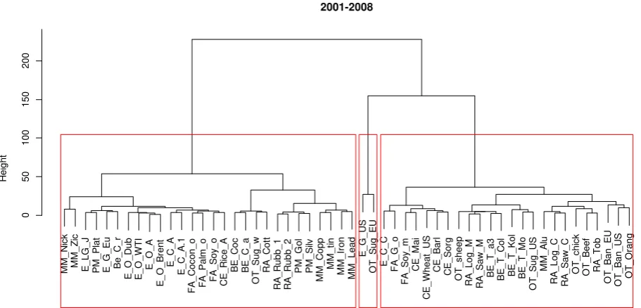
Figure 1 The classification results in the first sub-period

The results of clustering for the period 2001-2008 are presented in Figure 12, and they

yield three main clusters of time series (the average silhouette width is the biggest for three

clusters in Ward’s method – see Table 1). The first cluster consists of 28 commodity prices

including most energy commodities (their names in Fig. 1 begin with E), except for Gas US,

metals (MM), (except for aluminium), and precious metals (PM). What is more, commodities

belonging to the same category are close to each other, which means that their series paths are

quite similar. The prices from the categories listed above are closest to one another, which

means that their paths are the most similar. The second cluster includes the prices of Gas US

2

6 and Sugar EU, and it is hard to spot any connections between them. The last cluster consists

of 24 commodity prices including most food, raw materials and beverages commodities. The

silhouette plot indicates that most commodity prices have been assigned to proper

clusters(Fig. 4). Only in three cases, the silhouette width is negative, which means that objects

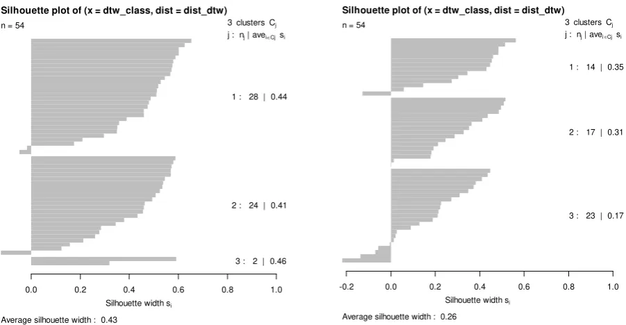
have been classified to improper clusters. Average silhouette width for this period equals 0.43.

F A _ G _ o C E _ B a rl C E _ M a i C E _ S o rg C E _ W h e a t_ U S R A _ L o g _ M B e _ C _ r C E _ R ice _ A E _ L G _ J F A _ S o y_ m E _ G _ E u E _ O _ A E _ O _ B re n t E _ O _ D u b E _ O _ W T I O T _ B e e f F A _ P a lm _ o F A _ S o y_ o M M _ ti n O T _ sh e e p P M _ G o l R A _ T o b B E _ T _ a 3 B E _ T _ C o l O T _ ch ick O T _ B a n _ U S R A _ L o g _ C R A _ S a w _ M O T _ B a n _ E U O T _ S u g _ E U R A _ S a w _ C B E _ T _ K o l O T _ O ra n g M M _ Ir o n M M _ C o p p M M _ L e a d M M _ Z ic P M _ P la t B E _ C o c B E _ T _ M o E _ G _ U S E _ C _ C M M _ A lu E _ C _ A E _ C _ A .1 P M _ S ilv F A _ C o co n _ o R A _ C o tt R A _ R u b b _ 1 R A _ R u b b _ 2 O T _ S u g _ U S M M _ N ick B E _ C _ a O T _ S u g _ w 0 50 100 150 2009-2014

hclust (*, "ward")

H

e

ig

h

t

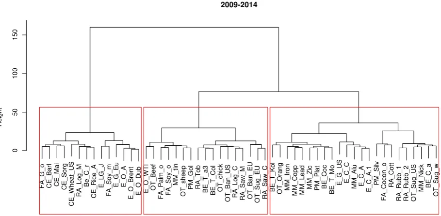
Figure 2 The classification results in the second sub-period

The results of clustering for the post-crisis period, with the assumption of Ward’s method,

are presented in Figure 2. Although in this case the average silhouette width suggests the

division into 2 clusters, we have opted for three cluster and, as a result, energy, metal, and

precious metals commodities are in different groups. There are 14 commodity prices in the

first cluster, including oil prices (except for WTI Oil, which is in the second cluster), some

food and raw material commodity prices. There are 19 elements in the second cluster,

including most food and raw material prices, gold, and tin. There are 23 prices in the third

cluster, including most precious metals, metals and minerals, coal prices and the remaining

food commodities. The silhouette plot (Fig.4) reveals that in the post-crisis period each cluster

is less homogeneous then before. Average silhouette for clusters varies between 0.17 to 0.35.

There are 5 commodity prices that seem to be classified to wrong clusters. Average silhouette

7 obtained is artificial.

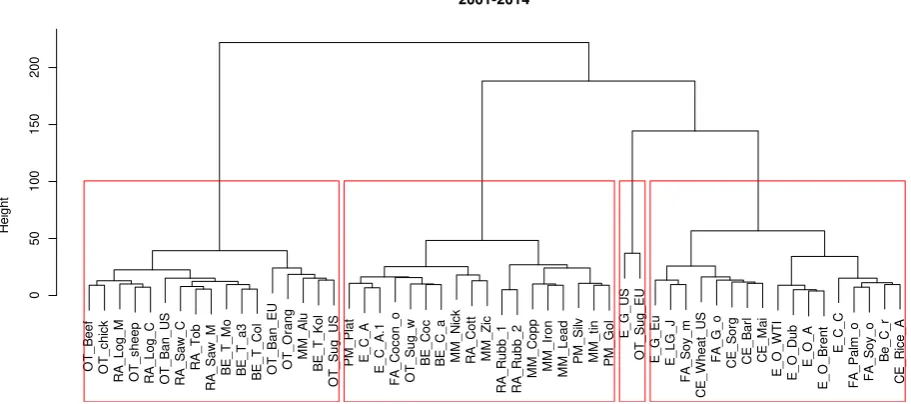
Finally, Figure 3 presents the results obtained for the whole sample. Here the average

silhouette width suggests (see Table 1) the division into 4 groups (although the quality of

division is rather poor). In the first cluster (17 elements) there are agricultural commodities

(beverages, raw materials and other) and one industrial metal – aluminium. In the second

cluster (18 elements) there are most industrial and precious metals, Australian Coal and some

other agricultural commodities. The last two clusters are quite close to each other. The third

consists of US Gas and Sugar UE, while the fourth contains most energy commodities and

some food, especially oils (palms, soya, groundnut).

O T _ B e e f O T _ ch ick R A _ L o g _ M O T _ sh e e p R A _ L o g _ C O T _ B a n _ U S R A _ S a w _ C R A _ T o b R A _ S a w _ M B E _ T _ M o B E _ T _ a 3 B E _ T _ C o l O T _ B a n _ E U O T _ O ra n g M M _ A lu B E _ T _ K o l O T _ S u g _ U S P M _ P la t E _ C _ A E _ C _ A .1 F A _ C o co n _ o O T _ S u g _ w B E _ C o c B E _ C _ a M M _ N ick R A _ C o tt M M _ Z ic R A _ R u b b _ 1 R A _ R u b b _ 2 M M _ C o p p M M _ Ir o n M M _ L e a d P M _ S ilv M M _ ti n P M _ G o l E _ G _ U S O T _ S u g _ E U E _ G _ E u E _ L G _ J F A _ S o y_ m C E _ W h e a t_ U S F A _ G _ o C E _ S o rg C E _ B a rl C E _ M a i E _ O _ W T I E _ O _ D u b E _ O _ A E _ O _ B re n t E _ C _ C F A _ P a lm _ o F A _ S o y_ o B e _ C _ r C E _ R ice _ A 0 50 100 150 200 2001-2014

hclust (*, "ward")

H

e

ig

h

t

Figure 3 The classification results in the whole sample period

methods Ward’s complete pam

period\nr cluster 2 3 4 2 3 4 2 3 4

2001-2014 0.235 0.287 0.322 0.605 0.265 0.322 0.274 0.196 0.225

2001-2008 0.374 0.427 0.301 0.746 0.423 0.274 0.382 0.429 0.301

2008-2014 0.371 0.257 0.221 0.378 0.237 0.221 0.338 0.245 0.214

8 Silhouette width si

0.0 0.2 0.4 0.6 0.8 1.0

Silhouette plot of (x = dtw_class, dist = dist_dtw)

Average silhouette width : 0.43

n = 54 3 clusters Cj

j : nj | avei Cjsi

1 : 28 | 0.44

2 : 24 | 0.41

3 : 2 | 0.46

Silhouette width si

-0.2 0.0 0.2 0.4 0.6 0.8 1.0

Silhouette plot of (x = dtw_class, dist = dist_dtw)

Average silhouette width : 0.26

n = 54 3 clusters Cj j : nj | avei Cjsi

1 : 14 | 0.35

2 : 17 | 0.31

3 : 23 | 0.17

Fig.4 Silhouette plots for pre –crisis (left panel) and post-crisis (right panel) period.

In order to compare the results of classifications, the adjusted rand index are computed (see

Table 2). The level of agreement of different classifications and the comparison of clusters

and categories of different commodities (listed in the World Bank indices – symbol WB in

table 2) are measured. As there are six different categories of commodities, the assumed

division of the set of objects also consists of six clusters.

period 2001-2014 2001-2008 2009-2014

WB ward compl. WB ward compl. WB ward compl.

WB 1 1 1

ward 0.100 1 0.139 1 0.077 1

compl 0.123 0.543 1 0.163 0.626 1 0.074 0.467 1

pam 0.167 0.415 0.496 0.125 0.588 0.688 0.114 0.490 0.569

Table 2 Adjusted Rand Index for different classification methods

The results obtained reveal that commodity classifications do not determine similar

behaviour of commodity prices, which is clearly seen in low values of ARI for the first and

the second (here the values are the highest) sub-periods as well as for the whole sample

period. As far as various methods of obtaining clusters are concerned, they are relatively high

(from 0.467 obtained for pair complete-ward in second sub-period to pair pam–complete in

9 sub-period, which indicates that in this sub-period co-movement of indexes is more evident,

and it is easily detected by different time series classification tools.

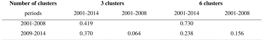
Number of clusters 3 clusters 6 clusters

periods 2001-2014 2001-2008 2001-2014 2001-2008

2001-2008 0.419 0.730

2009-2014 0.370 0.064 0.238 0.156

Table 3 Adjusted Rand Index for the ward results and different periods

In order to compare the composition of clusters in different periods, ARI index is

computed for 3 and 6 clusters. The results obtained reveal (see Table 3) that the composition

of clusters in pre-crisis and post-crisis periods differ greatly (in the division into 3 cluster ARI

equals 0.064 and into 6 clusters - 0.156). Relatively strong similarity of cluster composition in

the pre-crisis sub-period and the whole period (ARI from 0.419 to 0.73 for 6 clusters) results

from the fact that co - movement of all commodity prices in the pre-crisis period is stronger

and more evident.

4.

Conclusion and discussion

Dynamic time warping is used in the study to classify commodity price data in the

pre-crisis and post-pre-crisis periods. The results obtained reveal that co-movement of commodity

prices is more evident in the pre-crisis period when the clusters are more homogeneous and

consist of commodities from the same category (e.g. precious metals or energy commodities

are located in the same cluster). Clusters obtained for the post-crisis period are less

homogeneous. The internal classification measure demonstrates that the best division is

obtained if only two or three clusters are considered in every period. Clusters obtained for the

whole period sample indicate that there are only two patterns of behaviour of prices in the

periods analysed (stronger in the first one). Comparing commodity categories with the results

of clustering indicates that commodities which belong to one category do not always behave

in the same way. It is especially evident in the second period, when certain energy

commodities, metals or precious metals belong to different clusters. The results obtained

might be of great importance to investors, as they demonstrate that at present co-movement of

commodity prices is not as evident as it used to be. What is more, a well-diversified portfolio

10 Concluding our study, it can be said that co-movement of commodity prices is recently

not as evident as it used to be in the pre-crisis period. What might be the reason for such

change in the investors' behaviour? Of course, the lack of co-movement may result from the

disappearance of its causes, which include, according to popular explanations, low interest

rates and inflation expectations, shifts in global supply and demand, the risk resulting from

geopolitical uncertainties and speculative bubbles. The first two seem still valid. In the

post-crisis period real interest rates decreased. The post-crisis at first caused a dramatic demand slump,

which gradually came back to the initial level. Due to difficulties with direct measuring, it is

harder to refer to the remaining two causes of co-movement. It seems probable that the global

financial crisis has lead to increasing geopolitical risks, so it is justified to assume that

co-movement has been caused by speculations. Thus, it is most likely that the crisis has changed

investors' behaviour in the long run.

Acknowledgements

Supported by the grant No. 2012/07/B/HS4/00700 of the Polish National Science Centre.

References

[1] Alonso, A., Berrendero, J. Hernandez, A. & Justel, A., Time series clustering based on

forecast densities. Computational Statistics & Data Analysis, 51(2):762-776, 2006.

[2] Akram, F.Q.: Commodity prices, interest rates and the dollar. Energy Economics 31

(2009), 838-851.

[3] Berndt D., and Clifford. J., Using dynamic time warping to find patterns in time series.

KDDworkshop, Vol. 10, 16 (1994), 359-370.

[4] Byrne, J.P., Giorgio Fazio, and G., Fiess N.: Primary commodity prices: Co-movements,

common factors and fundamentals, Journal of Development Economics 101 (2013),

16-26.

[5] Frankel, J.A.: The effect of monetary policy on real commodity prices. In: AssetPrices

and Monetary Policy ( John Campbell Y.J., eds.), NBER, University of Chicago,

Chicago. 2008. NBER Working Paper 12713.

[6] Gilbert, C.L.; Speculative Influences on Commodity Futures Prices, 2006-2008, Working

11 [7] Gohin, A., and Chantret, F.,: The long-run impact of energy prices on world agricultural

markets: the role of macro-economic linkages. Energy Policy38 (2010), 333–339.

[8] Hubert, L., and Arabie, P.: Comparing partitions. Journal of Classification 2 (1) (1985),

193- 218.

[9] Irwin, S.H., and D.R. Sanders.: Index Funds, Financialization, and Commodity Futures

Markets, Applied Economic Perspectives and Policy33 (2011):1-31.

[10]Kaufman, L., and Rousseeuw, P.J.: Finding Groups in Data: An Introduction to Cluster

Analysis. Wiley & Sons, New York, 1990.

[11]Kilian, L., 2008. Exogenous oil supply shocks: how big are they and how much do they

matter for the US economy? Review of Economics and Statistics 90, 216–240.

[12]Kilian, L., 2009. Not all price shocks are alike: disentangling demand and supply shocks

in the crude oil market. American Economic Review 99, 1053–1069.

[13]Krugman, P., Commodity Prices, NYTimes, March 19, 2008.

[14]Kakizawa, Y., Shumway, R.H. and Taniguchi, M., 1998, Discrimination and clustering for

multivariate time series, J. Amer. Statist. Assoc., 93, pp. 328–340

[15]Kumar M., and Patel. N.R., 2007, Clustering data with measurement errors. Comput.

Stat. Data Anal., 51:6084-6101, August 2007

[16]Liao, W.,T.: Clustering of time series data—a survey, Pattern Recognition 38 (2005),

1857 – 1874.

[17]Natanelov, V., Mohammad, J., Alam, M.J., McKenzie, A.M., and Huylenbroeck G.V.: Is

there co-movement of agricultural commodities futures prices and crude oil? Energy

Policy39 (2011), 4971–4984.

[18]Nazlioglu, S, and Soytas, U.: Oil price, agricultural commodity prices, and the dollar: A

panel cointegration and causality analysis, Energy Economics34 (2012),1098–1104.

[19]Papież, M., and Śmiech, S.: The Analysis of Relations Between Primary Fuel Prices on

the European Market in the Period 2001-2011, Rynek Energii5 (2011), 139-144.

[20]Pindyck, R. S. and J. J. Rotemberg. "The excess co-movement of commodity prices",

Economic Journal, Vol. 100, (1990) pp. 1173-89.

[21]Phillips, P. C. B., and J. Yu.: Dating the Timeline of Financial Bubbles during the

Subprime Crisis. Cowles Foundation Discussion Paper No. 1770, Yale University, Yale,

2010.

[22]Svensson, L.E.O.: The effect of monetary policy on real commodity prices: Comment. In

Asset Prices and Monetary Policy. Ed. John Y. Campbell, NBER, University of Chicago,