Magnetohydrodynamic waves in structured atmospheres

Patricia M. Edwin

A Thesis Submitted for the Degree of PhD

at the

University of St. Andrews

1985

Full metadata for this item is available in

Research@StAndrews:FullText

at:

http://research-repository.st-andrews.ac.uk/

Please use this identifier to cite or link to this item:

http://hdl.handle.net/10023/2701

ATMOSPHERES

P. M.

EDWIN

A thesis submitted for the Degree of Doctor

inhomogeneities, on the magnetohydrodynamic (mhd) waves of an

infinite plasma is investigated. The appropriate dispersion formulae, in both Cartesian and cylindrical polar coordinate geometries, are derived. The main properties of the allowable modes in structured plasmas are described, particularly those featuring in a slender inhomogeneity.

The inclusion of non-adiabatic effects is examined, specifically for a thermally dissipative, unstratified, finite structure and for a slender inhomogeneity in a stratified medium. The dissipative time scales of slender structures are shown to have a dependence on the Peclet number. Growth factors appropriate to these time scales for

the overstable motions of a thermally dissipative, Boussinesq fluid are derived.

analogies are made with other ducted waves, for example, the Love waves of seismology. It is suggested that the behaviour of such waves, following an impulse, may account for the range of

oscillatory behaviour, the quasi-periodic and short time scales, observed in both the solar corona and Earth's magnetosphere.

Density variations across a structure and the structure's curvature, with possible applications to coronal loops, are also considered.

Further suggestions for possibly identifying some of the

me, and that it has not been submitted in any previous application

for a higher degree.

Signature of Candidate

degree of [loclor of Philosophy of the University of St Andrev:s and that she is qualified to submit this thesis in "'plication

for that degree.

Signature of Supervisor

October, 1980; the higher study for which this is a record was carried out in the Uni versi ty of St Andrevis between 1979 and 1984.

I am especially grateful to my supervisor, Dr Bernard Roberts, for his unfailing help, advice and encouragement during an extended and sometimes erratic period of study. I should also like to

thank Prof Eric Priest and past and present members of his Solar Physics group in St Andrews for many useful discussions.

I am grateful to The Open University for financial support and to my colleagues there for their understanding, encouragement and assistance, especially during periods of study leave.

My family, for their tolerance and sacrifices, I cannot thank enough.

Chapter 1

Chapter 2

Chapter 3

Introduction : Aspects of Structuring 1.1 Waves in Plasmas

1.2 Outline of Thesis 1.3 Structured Plasmas

1.3.1 The solar atmosphere 1.3.2 The Earth's magnetosphere

1.4 The Plasma Description Assumptions and Equations

Structuring in a Cartesian Geometry 2.1 Introduction

2.2 The Uniform Slab

2.3 General Discussion of Dis:eersion Relation 2.4 Incom:eressible Modes

2.5 Com:eressible Modes

2.5.1 Surface modes of a slender slab 2.5.2 The wide slab

2.5.3 Body waves

2.5.4 The field-free slab 2.5.5 Fast body waves

2.6 Detailed Nature of the Modes 2.7 Summary

Structuring in a Cylindrical Geometry 3.1 Cylindrical Structuring

3.2 The Uniform Cylinder

Chapter 4

3.4.1 Surface waves-solutions of Equation (3.20)

3.4.2 Body waves - solutions of Equation (3.21)

3.5 Non-evanescent Modes

3.6 A Slab/Cylinder ComEarison

Oscillations in the Corona AEElications and Analogies

4.1 An Overview

4.1.1 Observations 4.1.2 Theories

4.2 The Coronal Loop Model 4.3 Coronal Body Waves

4.4 Standing Waves in a Coronal Loop 4.5 Impulsively Generated Modes 4.6 Analogies

96

104

108 113

115

115 115 120 123 126 128 134 151 4.6.1 Waves on the lee side of mountains 152

4.6.2 Fibre optics 155

4.7 Density Variation in a Coronal Atmosphere 158 4.7.1 The slab

4.7.2 Cylindrical geometry

4.8 Further Features of the Optical Fibre .Analogy

158 175

Chapter 5

Chapter 6

4.9 Summary

Thermal Dissipation in a Structured Plasma 5.1 Dissipative Models

5.1.1 Introduction

5.1.2 Thermal time scales

5.2 Compressible, Gravity-free, Dissipative Modes

5.2.1 Radiative, non-conducting modes 5.2.2 Conducting, non-radiative modes 5.3 The Slender, Conducting Inhomogeneity 5.4 Gravitational Effects in a Slender,

Conducting Inhomogeneity

5.5 Structuring in a Thermally Dissipative, Boussinesq Fluid

5.5.1 The Boussinesq approximation 5.5.2 Thermal conductivity negligible 5.5.3 Dissipative effects

5.5.4 Slender structures 5.6 Summary

186 188 188 188 191 194 198 204 215 223 228 229 232 239 245 249

Nonlinear Effects : Slender Structures and Solitons 251 6.1 The Nonlinear Slender Tube Equations

6.2 Linearized Equations

Chapter 7

References

6.3.2 Discussion of the nonlinear, dispersive, dissipative equation 6.3.3 Compatability with linear,

incompressible, dissipationless theory 6.4 Solutions of the Benjamin-Ono-Burgers and

Related Equations

6.5 Modes in Slender Structures

274

276

280

285 6.5.1 Kink modes in a slender inhomogeneity 288

6.6 Summary

Further Applications and Conclusions 7.1 The Photosphere

7.2 The Chromosphere Waves in Fibrils 7.3 Structuring in the Magnetosphere

7.3.1 The plasma sheet

7.3.2 The cylindrical magnetotail 7.3.3 Comparisons

7.4 Laboratory Plasmas 7.5 The Corona Revisited

292

294 294 306 308 308 315 317 319 324

Chapter 1 Introduction Aspects of Structuring

'Within wave science as a whole~ the nature of waves in

fluids is characterised especially by their ability

to interact with complex ... fields.'

Sir James Lighthill 'Waves in Fluids'

1.1 Waves in Plasmas

A region of plasma such as the solar atmosphere or the Earth's magnetosphere can conceivably support several different types of wave. There are acoustic waves inherent in the medium because of the competing effects of compressibility and the plasma's own inertia. The latter may also form an effective balance with magnetic or

buoyancy forces resulting in compressible and shear Alfven waves, or internal gravity waves, respectively. In a magnetic, compressible and stratified medium these restoring forces may combine in such a way as to support magnetoacoustic-gravity waves, most of the other types of wave being deducible as special cases of this more general class of waves. (Inertial waves due to the Coriolis force in a rotating plasma are not considered here.) For an unbounded, uniform medium the theory of such waves, especially in the gravity-free case, is well-known (e.g., Landau and Lifshitz, 1960; Cowling, 1976; Lighthill, 1978; Priest, 1982). Small perturbations about an

iu.!t

according to e , then, for a uni form medium, w and k may be related by an algebraic dispersion relation. This relationship determines the phase-speed, w/k, the group velocity, 3w/3k, at which the energy is transmitted, and the dispersive properties of the wave. This theory, for a uniform medium, is valid if the wavelength 2n/k is much smaller than the length scale £ of the medium. Priest (1982) summarizes the properties of magnetoacoustic-gravity waves for a uniform plasma and points out the limitations of uniformity

assumptions for the solar photosphere where the length scale (the scale-height) may only be a few hundred kilometres.

these modes and to discover what other ne'" modes, if any, are present. In general the fact that there are no", discontinuities in the basic state, due to the inhomogeneities, leads to the existence of surface waves and the uniform medium waves are modified in the form of

body waves (terms to be defined in Chapter 2; see also Roberts, 1981 a,b). Having determined which modes the structured plasma can

support, the results are compared with observational data of oscillatory behaviour in the Sun's atmosphere and Earth's magneto-sphere to see whether explanations of such phenomena can be

offered.

1.2 Outline of Thesis

The remainder of this chapter reviews what is known of the inhomogeneities, and their wave-like properties, in two structured plasmas, the solar atmosphere and the Earth's magnetosphere. It

concludes with a summary of the equations which will be used. In Chapters 2 and 3 the dispersion relations for structures modelled in both Cartesian and cylindrical coordinate geometries are derived and their modes are examined both analytically and

modes along the structure. The main properties of the allowable modes in structured plasmas are described and the more important modes, in particular those featuring in a slender inhomogeneity, which has length scale small compared with the wavelength along the structure, are discussed in detail. In general the waves are dispersive and their existence is shown to depend on the form of the structuring.

For example, if the plasma of the Sun's corona is considered, two widely separated classes of free oscillation are possible, one on an acoustic, the other on an Alfvenic time scale. The acoustic-type oscillations always exist but the shorter period, Alfvenic-acoustic-type oscillations occur only in high density (low Alfven velocity)

structures. The latter waves are highly dispersive and are analogous to ducted waves occurring in several other branches of physics, in particular the Love waves of seismology (Love, 1911). The behaviour of such ducted, dispersive waves following an impulse has been

described by Pekeris (1948) in oceanographic studies. The fact that the phase-and group speeds of waves in structured plasmas have

periodic/quasi-periodic behaviour.

The form of the structuring need not necessarily be one due to a density inhomogeneity. As a result of the investigations of

Chapters 2 and 3 it is shown that similar ducted magnetoacoustic modes may occur in, say, the antiparallel magnetic field situations of the plasma sheet of the Earth's magnetotail (described in Subsection 1.3.2) or a coronal neutral sheet. Similar ideas to those of

Chapter 4 are thus employed in a different context in Chapter 7 to explain the variety of time scales and the wave-packet behaviour of magnetospheric observations. The deductions may also offer an alternative explanation for some of the coronal observations.

The Alfven and fast and slow magnetoacoustic modes of an unbounded, uniform medium arise from consideration of an ideal medium. When the medium is both dissipative and structured these modes are modified in a complicated way. In Chapter 5 the effects of thermal dissipation on the modes of a structured plasma are

examined, particularly with applications to the solar photosphere in mind. In this region of the solar atmosphere gravitational effects, too, cannot really be ignored and so they are also included in the analysis. If dissipation is present then for real k, w need no longer be real and the possibility occurs of overstability, that 1S

of there being oscillatory modes whose amplitude increases in time. The applications of these results are discussed in Chapter 7.

rise to the dispersion, that is it is due to the inertia and magnetic nature of the surrounding plasma. The importance of the dispersive nature of the waves in the context of group velocity is discussed in Chapter 4. For non-dispersive waves the idea of how linear theory can become inappropriate and waves steepen into shock waves is well established (see, e.g., Whitham, 1974; Lighthill, 1978; Priest, 1982). However if the waves are dispersive then it is possible for the

dispersive effects to counteract the steepening and a soliton or solitary wave results (see, e.g., Karpman, 1975). Further, if the dissipative effects also contribute to the effective balance then solitary waves with slowly decaying amplitude may result (see review by Kadomtsev and Karpman, 1970). In Chapter 6 the governing equation representing an effective balance between nonlinear, dispersive and dissipative effects is deduced and its solutions are shown to be solitary waves of slowly decaying amplitude. The possibility of such solutions describing spicular behaviour (see Subsection 1.3.1) or being applicable to the corona is discussed in Chapter 7.

1.3 Structured Plasmas

because of the mathematical analogies involved, waves occurring in other structured media, both in plasmas, such as the Earth's magneto-sphere, and those in optical fibres, for example, could not be

ignored. In turn ideas from the fields of oceanography, seismology and fibre optics contributed to the examination of magnetohydrody~amic

(mhd) waves in structured plasmas.

1.3.1 The solar atmosphere As far as the photosphere is concerned one of its most obvious features, the sunspot, has been known to be associated with magnetic field structuring since Hale's

spot and that it is cooled by overstable waves.

The sunspot does not present a homogeneous picture to the observer. Sunspots generally exhibit an irregular pattern of bright points, called 'umbral dots' (see reviews by Moore, 1981a,b), some

ISO km in diameter, with a brightness similar to that of the

surrounding photosphere and which have lifetimes of - 1500s. It is suspected that magnetic fields are smaller in these dots. Beckers (1981) has pointed out that there are no detectable intensity oscillations at periods of 1 to 300s as might associate mhd waves with these dots though 180s and 300s oscillations are associated with the sunspot umbra in general; periods of from 60 to 500s have been observed as well. For example, Lites et al. (1982) found evidence of 130 and 170s periods in sunspot oscillations which they suggested might be connected with magnetoacoustic waves. Athay (1981a) has

summarized the Ha (chromospheric) observations of sunspot oscillations. Briefly, there are thought to be vertical oscillations within the

umbra with periods ranging from 145s - 185s and horizontal penumbral -1

waves running outwards at speeds of 10 - 20 kms and periods of 210s, 270s or 300s. In his reviews Moore (1981a,b) quotes a range of 120 - 500s for umbral oscillations.

Sunspots apart, the rest of the photosphere is far from

homogeneous. Indeed Stenflo (1976) and Spruit (1981a) have described sunspots as being the largest members of a general class of magnetic

j1ux tubes, there being a spectrum of such magnetic flux elements

of elements in detail, from sunspots, through pores (- 2kG, 103km diameter), knots (1.5 kG, 500km diameter) down to the small (- 100km, 1500 G) concentrations of flux called variously flux elements,

magnetic elements or simply flux tubes. Indeed it is now generally accepted that the magnetic field over most of the solar surface is concentrated into regions of magnetic flux (see, e.g., Frazier, 1976; Stenflo, 1976) and that this accounts for over 90% of the flux seen by magnetographs.

Thus the sunspot may be considered as a large flux tube, or, as Parker (1974a, 1979c) has suggested it may be regarded as a cluster of flux tubes which perhaps separates into individual tubes at depths of 1000 km. A general overview of Parker'S model is given in the books by Noyes (1982) and Priest (1982). Intense tubes (knots of 1500 G) may assemble to form a sunspot from diffuse magnetic

fields. The latter are swept into the boundaries or corners of -1

supergranules by the strong downdrafts (- 1 kms ) depending on whether there is predominantly downflow, in which case the tube of field cools and the field strength increases and suppresses motion . . If there is upflow the field weakens and disperses. The flux bundle

idea is consistent with the umbral fields being nearly vertical (to within 10°) but becoming nearly horizontal at the outer boundary of the penumbra (Zwaan, 1981).

Roberts and Webb, 1978; Wilson, 1979; Roberts, 1981a,b; Spruit, 1982). Here it will be considered in the more general context of a structured plasma.

Of course, isolated flux tubes are at the limit of telescopic resolution so it is extremely difficult to detect oscillatory

behaviour within them. Athay (1981a) in discussing acoustic waves in the non-magnetic part of the photosphere/chromosphere points out the observational difficulties of distinguishing between waves, laminar flow and turbulent eddies, all of which would yield Doppler shifts. Giovanelli and Brown (1977) made the first observations of axial velocity fluctuations in gases in photospheric magnetic flux tubes and using the same observational technique Giovanelli et aZ.

(1978) provided further stimulating observations of such oscillations. Further observations, however, are very much needed but may have to await developments from space observatories (e.g., the planned Solar Optical Telescope experiment).

It has been suggested that flux tubes may act as a duct mechanism whereby wave information is transmitted from the Sun's interior into the higher solar atmosphere (see summary in Orrall, 1981). Stenflo (1976) stated as one of his main points that magnetic flux concentrations appeared to be cospatial with the photospheric and chromospheric network, that is 'pictures' of the Sun as seen from magnetograph observations seemed to fit those seen in Ha

o

much better picture of chromospheric features. Also it is generally agreed (e.g., Beckers, 1976, 1981; Harvey, 1977; Ramsey et a I., 1977; Athay, 1981b; Sheeley, 1981; Noyes, 1982) though evidence is incomplete, that the boundaries of supergranule convection cells correlate with the bright photospheric network and the chromospheric network (faculae and network clusters, and within them, filigree; see Dunn and Zirker, 1973) .

In turn,

spicules,

x

(several times the thickness of the chromosphere) and diameters typically 1" (725 km). I t is estimated (Athay, 1981b) that at any one time 1 to 2% of the solar surface has spicules, but that these are confined to the network, 'grouped like hedgerows' along the boundaries of supergranule cells (Noyes, 1982). Attempts have been

~

made to explain spicular behaviour by the buffeting of granule or supergranule cells on magnetic flux tubes thus causing waves (Parker, 1974c; Roberts, 1979; Hollweg, 1982; Roberts and Mangeney, 1982). One of the models, regarding a spicule as a soliton, is considered in Chapter 7.

in the H~photosphere of active regions as well as the bright and dark fine-scale mottles of the chromospheric network. He lists their properties; they have diameters of 1-2", lengths typically 10-15", lifetimes 15-30 mins and exhibit a range of velocities up

- 1

to SO km s . Marsh (1976) suggested that structural features such as spicules and fibrils carry (low temperature) matter along their lengths into regions where the ambient temperature is much higher. A canopy of spicule and fibril structure has been suggested

(Giovanelli, 1980; Athay, 1981b; Giovanelli and Jones,1982). There are many questions to be resolved concerning the chromosphere and the transition region. It is thought that the low chromosphere is affected by photospheric and sub-photospheric layers, but that probably the upper chromosphere and transition region are heated by conduction and convection from the corona and possibly by other processes (Hollweg, 1981). It is not clear however whether it is the magnetic field structure or the temperature

structure which "calls the tune".

Observations of chromospheric oscillations are limited (Liu, 1974; Beckers and Artzner, 1974; Giovanelli, 1975; White and Athay, 1979; Athay and White, 1979; Giovanelli and Beckers, 1983). Periods in the range 100-500s are quoted, sometimes down to 30s. Often reference is made to "the 5 min photospheric and the 3 min chromo-spheric" oscillations (Leibacher and Stein, 1981). (As far as the photosphere is concerned these 300s oscillations have been identified

resonant subphotospheric cavity.) Waves are thought to be upwardly propagating wi th velocity amplitudes 1- 3 km s -1 and phase-speeds on

-1

the order of the sound speed (- 7.5 km s ) (Athay, 1981a).

Giovanelli (1975) has described the propagation of waves in chromo-spheric fibrils. A suggested explanation of these fibril waves is glven in Chapter 7.

As a result of increased coronal knowledge, especially via the EUV and soft X-ray observations of the Skylab mission, epithets relating to this part of the solar atmosphere abound - magnetically dominated, paramountly inhomogeneous, inherently structured, highly conducting, arch-like, extremely hot -and from this list a picture has emerged that is one of a highly inhomogeneous medium structured almost entirely by loops. Webb, D.F. (1981) has drawn the

distinction between the flux loops (isolated tubes of magnetic field surrounded by a relatively field-free medium discussed above) and the plasma loops of the corona, the observed emitting structures which seem to act as coronal magnetic field tracers.

There are loops large and small. Even the tiny X-ray bright points of ephemeral regions which have time scales of the order of

Y3

magnetically opposite footpoints in the denser chromosphere and photosphere, and some appear to be hot and dense themselves,

observable because of their X-ray emission (Webb, D.F., 1981; Zirker, 1981). These closed loops, on average, extend no higher than half a solar radius (R

=

(3

'open', fading high in the corona. They may emanate from coronal holes, which (at a height of about lR ) are the cooler (1.5 xl05_K

13

6 14 -3

rather than 2 x 10 K) and less dense (- 7% of the 5 x 10 m 'normal' particle density at this height.) regions of the corona, or they may form part of the 'helmet streamers' (see Figure 1.1 and descriptions in Spicer and Brown, 1981; Priest, 1982). Following a sunspot

maximum these streamers have been seen to extend as far as l2R

o

from the Sun (Noyes, 1982).

Because of the large variation in size and type of loop their properties vary considerably. An attempt has been made at a

classification into 'hot' and 'cool' loops (Orrall, 1981). Webb, D.F. (1981) quotes field strengths of 300G and suggests that brightness variations over the loop imply density variations. Wentzel (1981) gives a value of 100G for small, compact loops,

.,. 3 -1

and a typical Alfven speed of 3 x 10 km s . He suggests that loops are not homogeneous but that they may be composed of several flux tubes with different gas pressures. Suggestions have been made that some loops have cool cores (Foukal, 1975, 1976; Jordan, 1975; see also Levine, 1981). The particle density appears to vary according to the model but values ranging from - 1.6 xl016_m-3 _{on the axis of}

...c

o

en

o

- - '

6-

4-/1

fi bril

)

. )1

closed

coronal loo ps

I

-!drlr-- --

-

~i'

---

"~

t~.ti

/ ---

---

)d~

/ -

--- photospheric flux tubes -

~

-,."..

-

- -

-Fjgure 1.1 A schematic picture, varying logarithmically with height h (km) showing solar atmospheric features.

Compiled from similar diagrams in Stenflo (1976), Withbroe and Noyes (1977), Parker (1979a), Spicer and Brown (1981), Noyes (1982) and Spruit (1983).

'I'

review by Jordan (1975). Pick et al. (1979) analysing a coronal structure overlying an active region estimated it to be about 10

times as dense as the background corona and Spruit (1981a) suggests the coronal tube density may be higher than its environment by a factor of 3-10. These values usually refer to loops in active regions being the easier ones to observe. In Chapter 4 an attempt to model such inhomogeneity will be made by considering loops having transverse density variations. It must be added that loops are often observed to be twisted. The stresses and instabilities resulting from twisting motions are often essential ingredients of theories for coronal heating. Here, however, loops will be assumed to be free of twist; wave-like behaviour, rather than instabilities, will be investigated. Some of these coronal loops are more evident shortly after a solar flare: the 'post-flare' coronal loops.

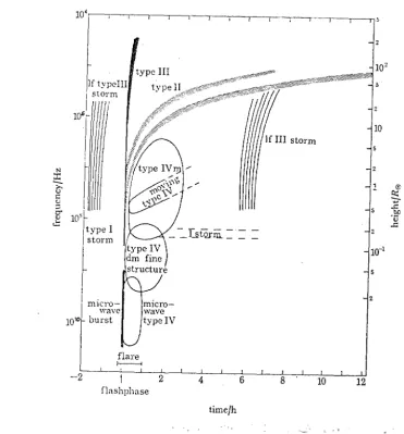
Information concerning the oscillatory behaviour of the plasma following a flare comes from radio wave data (Kruger, 1979) and more recently from the hard X-ray data of the HXRBS (Hard X-ray Burst Spectrometer) of the Solar Maximum Mission satellite (e.g., Kiplinger, 1983a,b). There is also some coronagraph evidence of oscillations (e.g., Koutchmy et aL, 1983; Pasachoff and Landman, 1984). The radio wave data has a complicated categorization (see review by Rosenberg, 1976 and Figure 1.2). Briefly, the Type I and IV data is thought to originate within the region of the explosion itself, as a result of interacting energetic matter and the magnetic fields, the Type III bursts being rapidly upward-propagating

N

::c

>: _u

t:

'-'

0-u

t.':::

Figure 1.2

type III

If typeIII storm

wr

1

II

lo,L

Itype I

l'to'm

I

micro-wave

1010 _burst

flare

l---I

-2 2 4 6 8 10 12

flashphase

timefh

Schematic representation of the radiospectrum after Rosenberg (1976). The Type I and tf (low frequency) Type III storms are not necessarily flare-related.

not be considered here. In Chapters 4 and 7 models of both open and closed coronal loops will be considered in an attempt to explain the diversity of periodicities, from seconds to minutes, especially the shorter - Is periods observed in the corona. Most oscillatory

As a result, then, of information gained over the past decade or so, particularly from Skylab, a picture of the solar atmosphere has evolved (Parker, 1979a; Noyes, 1982; Spruit, 1983) that more or

less represents current thinking as to the atmosphere's structure (Figure 1.1). Photospheric flux tubes are imagined to fan out so that their outer boundaries become more horizontal and tubes merge

(e.g., Parker, 1979a; Sheeley, 1981) the coronal tubes (loops) possibly being related to flux tubes as shown in Figure 1.1. At what height this occurs is subject to debate. Spruit (198la) suggested that the 'interface' between the photospheric flux tube regime and that of the coronal field occurs at about 1500 km in a quiet region and at about 750 km in an active region, whereas Giovanelli (1980) proposed that the chromosphere/corona transition region probably penetrates below 600 km. In a later paper

(Giovanelli and Jones, 1982) the canopy height was estimated to be even lower, - 300 to 400 km, certainly much lower than the static

displaced laterally some hundreds of ki lometres originating, say, in the quiet photosphere and following the line of a coronal

streamer. In order to relate the magnetic inhomogeneities with the emission inhomogeneities (those due to differences in temperature, say) Spruit (198la) and Zwaan (1981) amongst others, have described the idea of a

filling factor,

It must be noted that though the overall features of the Sun's atmosphere are often described in terms of the plasma S, the ratio of gas to magnetic pressures, this can often be misleading. In the corona, which is magnetically dominated, it is generally accepted that S « 1 and the 'cold plasma' approximation, or neglect of sound as compared to Alfven speed, is an acceptable simplification there.

-4 -1

(Spruit (1981a) suggests S - 10 -10 in the lower solar corona.) However, as Figure 1.1 shows, a description of the photosphere may vary from S ~l, in the vicinity of an isolated flux tube or sunspot say, to S » 1, In a relatively field-free region.

This idea will be used extensively, but especially in Chapter 6. It is perhaps a weakness of the modelling that no attempt is made to impose boundary conditions at the 'ends' of these structures and thus relate the various levels of the solar atmosphere. However as regards the coronal oscillations discussed in Chapters 4 and 7, an initial value problem is discussed and conditions on transverse boundaries become less relevant.

As far as the photosphere is concerned the inhomogeneities will be assumed to be those due to magnetic structuring (flux tubes, sunspots), whilst structures in coronal regions will primarily be thought of as density inhomogeneities - though apart from a brief section of Chapter 4, which deals specifically with density variations these are just differences in Alfven speed and could incorporate

structuring due to pressure, or temperature, or magnetic field strength as well.

Thermal conduction effects are considered in Chapter 5 with the magnetically structured inhomogeneities of the photosphere in mind. Spruit (1977) has argued that thermal conductivity in the environment of a sunspot is very large so that the missing flux is spread out over an area several hundred thousand kilometres in diameter. An attempt is made in Chapter 5 to include two important photospheric features in the flux tube models, those of (constant) thermal dissipation and gravity.

considered here. The possible waves inherent in the solar atmosphere have proved to be a topic enough in itself; waves mayor may not be contributory factors in heating and acceleration mechanisms

associated with magnetic fields (see summary by Hollweg, 1981). However it must be emphasized that considerations of mhd waves,

coupled with the fact that the corona is highly structured magnetically have led to a resurgence of interest in coronal heating mechanisms. Several ideas have been proposed. Ionson (1978) suggested exploiting a resonance mechanism (see Section 2.1) to produce so called

'dissipationless' damping and this was further investigated by Rae and Roberts (1981, 1982). The idea of enhancing dissipation (and thus heating) by phase mixing of shear Alfven waves has been proposed by Heyvaerts and Priest (1983) and followed up in more detail by Browning and Priest (1984) and Nocera et al. (1984). This work concentrates on the dissipation mechanism due to Alfven velocity gradients within the corona. Hollweg (1984), on the other hand, concentrates on how energy can be carried from the convection zone to the corona, by waves, and considers a coronal loop as acting as a leaky resonant cavity. Ideas based on wave transport mechanisms have been extended to include not just the corona but the solar wind as well (e.g., Hollweg, 1978, 1983; Habbal and Leer, 1982).

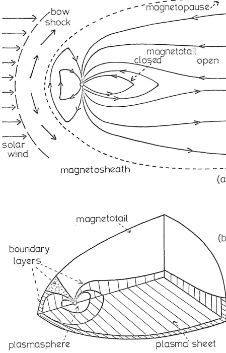
1.3.2 The Earth's magnetosphere Another instance where structuring in a plasma is of importance is that of the Earth's magnetosphere. Excellent descriptions and summaries of current thinking regarding the magnetosphere's structure have been given by Vasyliunas (1983) and those features relevant to the discussion here are illustrated in Figures 1.3a and 1.3b. Near the Earth and on its daytime side the structure is thought to be very complicated, a bow shock and magnetospheric boundary layers forming where the solar wind interacts with the Earth's magnetic field, the boundary layers funnelling down towards the earth in the form of polar cusps and relating to the auroral zones.

Two parts of the magnetosphere morphology are, however, well defined. The first is the magnetopause surface 'separating' the magnetosphere itself from the magnetosheath. It is some tens of Earth radii (Re ~ 6 xI03_{km) in extent and encompasses the region of}

both closed and open magnetospheres, some field lines of the latter being able to form the connection between the Earth and the solar wind (Figure 1.3). The second well-defined region is the magnetotail or geomagnetic tail lying downstream (in the solar wind sense) of the closed magnetosphere, being a region of reversed magnetic field between the extended field lines from the northern and southern hemispheres of the Earth. McKenzie (1970) modelled the magnetotail as a cylindrical tube some 20Re in radius (- 2 xl05km diameter).

Extending earthward through the centre of the magnetotail lies the hot plasma sheet. In turn, through its centre lies the neutral

boundary

layers~

\ " ~

\

"

I

plosmosphere

~--­

---(a)

magnetotail

" "

(b)

"

plasma'sheet

extends across the magnetotail in the form of a slab. McKenzie (1970) adopted this latter view and it is one of the models which will be considered in Chapter 7. Galeev (1982) takes the half-width of the plasma sheet to be just 1 Re. On the other hand, Patel

(1968a,b) modelled the magnetic tail as both a cylindrical (radius - 7Re) hydromagnetic waveguide and resonator neglecting the plasma sheet which he supposed to be of thickness 4 - 6Re. Contrast the lengths used by Patel (- 25,40,50 and 100Re) with that of 220Re being used some 20 years later by Hones et al.. (1984) who are

investigating satellite measurements in the plasma sheet at such a distance from the Earth.

In Chapter 7 the plasma sheet will be considered as a hot plasma slab with half-thickness some few Re and infinitely broader and longer than its thickness.

The magnetopause, the plasma sheet and the flow pattern within it have all been observed to exhibit systematic temporal variations

(see reviews by Hughes, 1983; Southwood and Hughes, 1983). Evidence comes from both ground-based and rocket and satellite observations

in the 1850's following a large solar disruption. Hughes (1983) describes geomagnetic pulsations as being the 'ground signature of hydromagnetic waves in the atmosphere'. However there are difficulties of interpretation of magnetometer data because of the effect of the ionosphere, which, if it is assumed to be a finitely conducting horizontal layer between the magnetosphere (where mhd solutions pertain) and the Earth's insulating atmosphere, probably reflects waves from its upper surface, the magnetic field observed on the ground being due to the ionospheric Hall current (Walker et aI.,

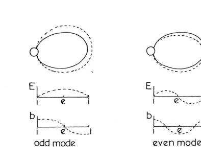
1979; Hughes, -1983; Southwood and Hughes, 1983). In the former reference, and also in Greenwald et al. (1981), these conclusions result from attempts to correlate the STARE (Scandinavian twin auroral radar experiment) auroral radar data with both GEOS2 (a geostationary satellite) data and geomagnetic pulsations from ground-based magnetometers. The arguments in these papers are based on models of field line resonances (Chen and Hasegawa, 1974a; Southwood, 1974; see also Section 2.1) illustrated in Figure 1.4, in which the Earth's (dipole) magnetic field is anchored in the ionosphere and , standing waves are set up on the finite length field lines. However such models usually assume that the plasma is cold which, as

Lanzerotti and Southwood (1979) and Hughes (1983) point out, is

Figure 1. 4

, - - -

--...

---

.

e

.

I

I

i

e", - ___

j

odd mode

- - - - '

b

t""

-i

e ,,,'

---even mode

Following Southwood and Kivelson (1981) an idealized picture of geomagnetic field line oscillations assuming a perfectly conducting ionosphere (i). e: equator; -- : unperturbed field; ---: perturbed field;

E : electric field; b: magnetic field perturbation.

of the magnetosphere forming some sort of duct. He hints that surface waves are important. Such waves are described in Chapter 2 and used in magnetospheric models in Chapter 7.

The origin of oscillatory behaviour lS open to much speculation.

bow shock or from the turbulent magnetosheath or more subtly via various plasma instabilities in the form of sharp spatial gradients, temperature anistropies, etc. The literature seems almost purposefully vague! Chen and Hasegawa (1974b) refer to pulsations being excited by sudden commencements and sudden impulses near to the magnetopause' and Lanzerotti et al. (1973) refer to unknown impulse sources which excite mhd surface waves at the plasmapause.

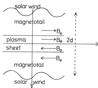
In an attempt to represent the effects of the solar wind on the magnetotail, another series of models was developed (Siscoe, 1969; McKenzie, 1971) which considered a geometry as shown in Figure 1.5, with the solar wind being represented as a (usually sinusoidal) driving force acting on the magnetopause x = ±d. Of course these models presume the magnetotail and its embedded plasma sheet to have almost constant thickness. However analyses of satellite data and related theories (e.g., Mihalov et a~, 1970; Forbes and Priest, 1982; Hones et a~, 1984) suggest variations in sheet thickness as plasmoids are formed and spontaneously released near the Earth, possibly as a result of magnetic reconnection.

Figure 1.5

magne otail

>B

_e

plasma

>8

2d

sheet

8

0

<

Be

magne

o tail

I I

V

x

The magn~totail geometry of Siscoe's (1969) and

McKenzie's (1971) models.

basically the models are similar to those considered by McKenzie (1970). However one feature of oscillatory behaviour occurring in observations, from both space and ground-based stations, is the apparent wave-packet structure (Mier-Jedrzejowicz and Hughes, 1980) or 'decay' of a train of oscillations (Walker et

at.,

z

the solar atmosphere and the magnetosphere without qualification. Similarly mhd waves have been mentioned without any reference to what is meant by an mhd model. Here Goedbloed's (1983) attitude is

adopted, of postulating the equations of mhd for a hypothetical medium, 'a plasma', to describe the interaction of a perfectly conducting fluid with a magnetic field. Whilst recognizing that the area of validity of such a model is limited (for example, Wentzel

(1981) has warned about inappropriate models for coronal heating theories and Southwood and Hughes (1983) stress the limitations for the magnetospheric problem) it seems only sensible to proceed with the universal idea of a continuum description that is so well-known and well-used (e.g., Landau and Lifshitz, 1960; Roberts, P.H., 1967; Cowling, 1976; Parker, 1979a; Priest, 1982; Goedbloed, 1983).

S.I. (rationalized MKS) units will be used throughout except for brief comparisons with observations in Chapters 4 and 7. The symbols used in the following for the plasma's scalar and vector fields are

P

p

B

It will be assumed that the medium under consideration is a perfect (electrical) conductor so that Maxwell's equations may be combined to give the mhd induction equation,

dB

Using one of Maxwell's equations,

div

B

and the divergence theorem, the mhd analogue of Helmholtz's theorem, namely

Is

B.

where S is a flux tube cross-section, may be derived. This, of course, states the 'frozen-in' condition for perfect conductors.

Other mhd equations which will be referred to throughout this thesis are listed below.

The equation of continuity (conservation of mass) is

dp

- + p divv

dt 0,

d _ 3

where dt = 3t + v . grad is the (total) Lagrangian differential (1. 4)

operator, and the equation of motion (conservation of linear momentum) is

dv

p

dt

=

1-10

(1. 5)

2 -2

where g is the gravitational acceleration (of magnitude 2.74 xlO ms ). Here isotropic constitutive equations have been assumed in order to

combine Maxwell's equations and 1-10 is the magnetic permeability of

the plasma, taken equal to the constant value of that of free space

-7 -1

Neglecting the rate of heat generation internal to the fluid -1 -1 -1 and assuming the heat transfer coefficient,

Q

dT

dn_

pc - - - ~

QV2T - R

p dt dt- (1. 6)

where c is the specific heat at constant pressure per unit mass,

p

and the radiative loss term, R, will be assumed to obey Newton's law of cooling (see Spiegel, 1957; Bray and Loughhead, 1974) and have the form

R

pc

v

TR (1. 7)

Here, To is the ambient temperature of the plasma, c the specific v

heat at constant volume (per unit mass) and TR is the radiative relaxation (decay) time which will be assumed known from tables such as those in Bray and Loughhead (1974), Spruit (1974) and

Giovanelli (1978).

If the plasma is assumed to be a perfect gas, then

p =

RpT,

where R is a constant for the gas (equal to c

p - Cv or kB/m where kB is Boltzmann's constant and

m

3 2 -2 -1

In much of the thesis only the linearized version of the above equations will be used. It will be assumed that there is an

equilibrium state (v =0) in which variables have the values Po' Po'

To

(1. 9)

and (1. 6) gi ve s

(1.10)

while (1.2) gives

~.~o =

O.

If ~ and [ are typical time and length scales for the system under consideration then T = [2/K is a typical diffusion time. Here

K

K =

is the (constant) thermometric conductivity or thermal diffusivity 2 -1

(m s ). If t « TK,T

R then the terms on the right-hand side of (1.6) may be neglected and the resulting equation describes adiabatic (isentropic) flow. For adiabatic flow, using (1.8), Equation (1.6) reduces to

where y ::: C

Ie ..

p v

~_l£dp

If the gravitational force g and the equilibrium magnetic field

~o are assumed to act in the +z directions respectively (for the Cartesian and cylindrical polar coordinate systems used in this thesis), then the transverse component of the equation of motion

A

(1.5) in the n direction (where n is x or y or r, a unit vector

-s -s

orthogonal to the z direction) implies that

a

an

s

whilst the vertical component gives

(1.13)

(1. 14)

If p, p, ~ and ~ are the (small) perturbations in density, pressure, magnetic induction and velocity fields, respectively, about

corresponding equilibrium values, so that

p

=

c~

(1.1) and (1.11) give

ab

at

and (1.4), (1.5) and (1.12) become,

ap

- +

at

av

(

Po -;:;-t - -IJ P + - Bo.bJ + (B_o·IJ_)~ + - (~·~)~o + pg

and

(1.18)

Generally gravitational effects wi 11 be ignored (g = 0) except for Chapter 5 when this term will be retained to provide a better model of the lower solar atmosphere.

The boundary conditions across a surface of discontinuity, which may be derived by integrating (1.4), (1.5) and (1.6) across the surface (see, e.g., Roberts, P.H., 1967) or in the case of

(1.20) by examining perturbations of the transverse momentum equation about the basic state (Roberts and vlebb, 1978) and which will be used throughout are that:

the transverse (normal) component of velocity is continuous, (1.19)

and

the total perturbed pressure, PT P + BObz is continuous,

]..lO

the transverse heat flux K

~

the temperature perturbation T is continuous.

(1. 20)

(1.21)

(1.22)

Chapter 2 Structuring in a Cartesian Geometry

'With a name like yours3 you might be any shape3 almost.'

Lewis Carroll ' Through the Looking Glass'

2.1 Introduction

In order to examine structuring in the plasma it will be assumed first that the structure can be considered in a Cartesian geometry which has infinite extent in the z-direction (of a Cartesian

coordinate system xyz). The effects of stratification due to gravity will be ignored. In the equilibrium state it is supposed that the plasma pressure PO, density

Po

Linear, isentropic perturbations about the basic state then obey equations (1.15) to (1.18) with ~ ==

2.

r

- z

and PT == P +

~

Vo z x y z - x y z

perturbation equations, (1.15), (1.16) and (1.18), may then be written:

~== -p 0 c02~ - v ~

at x dx ' (2.1)

ab av

x

Bo

at az

,

ab av

-L

_{Bo -L}

at az

,

ab

- v

(~)

z

Bo (r - /':,)

and

at

where, in (2.3), the fact that there is total pressure (gas plus magnetic) balance in the basic state (see Equation (1.13)) has been used, that is

d [ B 21

dx Po +

2~oJ

o.

k ~

Here vA(x) = (B02/~OPO)2 is the Alfven speed and co(x) = (YPo/Po) the sound speed.

The equation of motion (Equation (1.17)) may be differentiated partially with respect to time and variables other than v eliminated to give (see Roberts, 1981a)

(2.S)

(2.6)

and

(2. 7)

Equations (2.1) through (2.7) may now be Fourier analysed by writing the variables in the form

v x

A ( ) i(wt+£y+kz)

v x e ,

x

A ( ) i(wt+£y+kz)

PT x e , etc., (2.8)

and after some manipulation it is found that the x-dependent amplitudes of the perturbations, Vx and

P

equations

(2.9)

and

dv _{x _} 2 2 2 2 2 2 2 2 2 2 2 2 A

W[(k VA(X)-W ) (k Co(X)-W ) +£ (k CT(X)-W ) (Co(X) +VA(X))]PT

dx - _{. 22 2 2 2 2 2 2}

1 Po (x) (k vA (x) -w ) (k c_T (x) -w ) (cO (x) + vA (x))

(2.10)

where

c~(x)

2 2

Co (x)v A (x)

2 2

Co (x) + vA (x)

(2.11)

Equations (2.9) and (2.10) may be combined to glve

where

~

(k2v~(x)

d _{x mo (x)} 2 _{+ £} 2 - d -_x Po (x) [k VA (x) - W ] v _x - 0,

2

mo (x)

(2.12)

(2.13)

Equation (2.12) is the Cartesian equivalent of the Hain-Lust equation

(Hain and Lust, 1958), arising in a cylindrical geometry, which is

discussed in Chapter 3. It has been obtained by, for example, Goedbloed

(1971), Chen and Hasegawa (1974b), Wentzel (1979a) and Roberts (1981a).

If there is no structuring of the medium, so that coefficients

in (2.12) are independent of x, then this equation simplifies to

ikxx

which, for an x-dependence of the form e ,gives

o.

The assumptions made in deriving (2.15) mean that a uniform, infinite medium is being modelled. Rewri ting (2.15) by substituting for m2 _o shows that its roots are the well-known Alfven modes

(2.16)

and magnetoacoustic modes,

(2.17)

of a uniform medium (e.g., Cowling, 1976). The aim in this chapter is to investigate how these modes are modified by the x-dependence

introduced by the structuring of the medium. If the structuring is weak, in the sense that the factors in (2.12) vary only slightly with x, then a local approximation may be made, with (2.16) and (2.17) giving the appropriate modes.

If the medium is considered both uniform and finite, by the introduction of rigid boundaries, say, at x = ±xo, then the wavenumber k (for £ and k fixed) is quantized by being an integer, s times TI/2xo,

x

where s relates to the number of nodes of the eigenfunction v (the x transverse velocity). Goedbloed (1983) points out that such a labelling of the discrete eigenvalues still makes sense in an inhomogeneous medium when the equilibrium quantities vary in the x-direction. To demonstrate his idea he considers the limit k ~ 00

(s + 00) in Equations (2.16) and (2.17) and lists the essential features

of the spectra of eigenvalues, w2, resulting from this limit, as being:

(i) the infinitely degenerate point eigenvalue, w2 ==k 2v2

A'

(ii) the cluster (or accumulation) point, w 2 2 2 2 2 +k c v / (c + v ), 2

DAD A

and (iii) the cluster point, w2 + CD •

Goedbloed goes on to show that these three facts facilitate a division

of the inhomogeneous case, with its associated singularities, as is

discussed below.

The singularities of Equation (2.12), in both Cartesian and

cylindrical geometries, have been the subject of much discussion,

since at these points it is known that in the presence of dissipation

the plasma can absorb energy from some external forcing mechanism

and cause resonant heating (see, for example, Southwood, 1974;

Hasegawa and Chen, 1974, 1976). Most of the discussion in the

literature has concentrated on the incompressible

(m~(x)

two-dimensional (R, == 0) form of (2.12), in which the resonance occurs

at the singularity w2 ==

k2v~(x),

matches the local Alfven speed, vA(x). Sedlacek (1971) attempted to

reconcile the different mathematical behaviour resulting from a

continuous vA(x) profile, which gives a continuous spectrum of modes,

and that resulting in discrete modes which arise when the medium is

uniform and thus the factor (k2vi -w2) is removable from (2.12). Lee

(1980) and Rae and Roberts (1981) pointed out, however, that

Sedlacek's results have been wrongly interpreted by Jonson (1978)

0

incompressible medium.

Extending consideration of singularities of (2.12) to a

compressible medium, Rae and Roberts (1982) have shown that as well

as the Alfven singularity there is the important cusp singularity

where w2 = k2c~(X). (See also fact (ii) of Goedbloed's classification

above.) As Appert et aZ. (1974) have pointed out, in their discussion

of a cylindrical geometry, these singularities are more evident from

the first-order equations (2.9) and (2.10). Goedbloed (1983) has

helped clarify the nature of the differential equation (2.12) by

expressing the first term as

where

The structure of (2.12) is then illustrated, following Goedbloed

(1975, 1983), in Figure 2.l. Goedbloed has emphasized that {wI} 2 and

C.p.

Cp.

{w~l

Cp.

c.p.

t~~J

c.p

\

J

'IN'-

~

I

'lfl.f\

1-)( )( _1'U III

"

)( ,.>

W

{kLC~}

_[k

v;-}

Figure 2.1 Schematic representation of the singularities of

Equations (2.12), after Goedbloed (1975, 1983)

~: spectrum 'separators'; x: discrete modes;

2

{w₂} are not part of the spectrum (note that they are the roots (2.17)

in a

uniform

subspectra. Separation only obtains if the inhomogeneity is weak.

However, a detailed analysis, such as Sedlacek's, of the behaviour

of the compressible modes near these singularities, where the

transition from discrete to continuous spectra takes place, has not

been carried out.

Discussion of (2.12) in its general form is, unfortunately, a

difficult task and though x-variation will be considered to some

extent in Chapter 4, here it will be assumed that the non-uniformity

of the medium takes the form of a uniform slab of discontinuity (say

a magnetic field or density rapidly varying in the x-direction) which

is infinite in the y-direction, so that

v

y

Of course, as Parker (1979a) has pointed out, such a slab geometry

(especially if of infinite extent in the y-direction) will offer

much more resistance to any changes in the slab exterior than, for

example, an inhomogeneity (such as an intense magnetic flux tube)

represented by a cylindrical structure. However, in order to try

to elucidate the behaviour in a structured situation, it was decided

to examine the simpler Cartesian geometry first. A cylindrical

geometry is investigated in the next chapter and compared and

2.2 The Uniform Slab

z

Figure 2.2 The equilibrium configuration

In Figure 2.2 the basic state of the plasma is one in which

the pressure, density and magnetic fields are uniform inside a slab

of width 2xo and also have uniform (but not necessarily the same)

values in the slab's environment. Thus, in the equilibrium state,

(2.18)

and Equation (2.4) shows in this case that

B 2 Be 2

p +.:::..L. = p + _ _

o

Using expressions for the sound and Alfven speeds in the slab's

environment (Ixl > xo) c! = YPe/P_e and v}e =

2

together with the equivalent ones for Co and

be expressed in the alternative form

Pe

- =

Po

B2/~Op , respectively,

e e

v1, Equation (2.19) may

Since the plasma has now effectively been split into two

uniform media, the slab interior (Ixl < xo) and its environment

(Ixl > xO), perturbations about the equilibrium (2.18) to (2.20) are

described, for the transverse velocity amplitude, by Equation (2.12),

where the coefficients are now constants for each region. Inside

the slab,

(2.21)

where

(L.2vi - w2) ( k2c

t -

(c 0 + vA)(k c_T - w )

(2.22)

Also, for i = 0 and v = 0 (so that there is no variation in the

y-y

direction) Equation (2.10) gives

. (2 2)

1Po Co + vA

w

dv

(2.23) dx

and Fourier analysis of Equation (2.7) shows that

(2.24)

Now observations of oscillations in structured plasmas are

limited, but there is evidence, for example in the case of

chromospheric fibrils (Giovanelli, 1975) and the magnetospheric

plasma sheet (McKenzie, 1970) that oscillations are confined mainly

to the inhomogeneity. In other words, the inhomogeneity appears

slab I S exterior,

I

I

that

v

I

I

x

solutions which result when this assumption is not made is deferred

until Chapter 3 (Section 3.5).

In this case the appropriate solutions of Equation (2.21) in

the slab and its exterior can be described by:

-me (x-x o)

Q:e

e

,

V

x

me (x+xo)

x <

Be e

,

-xo,

where 0:0, _{So, Q:e and Be are arbitrary constants and me is given by}

(2.26)

The assumption of lateral evanescence restricts me to be positive.

The four constants in (2.25) are evaluated by invoking the

boundary conditions, Equations (1.19) and (1.20). These establish

continuity across the two boundaries, x

=

transverse (normal) velocity

v

x

PT(x). For a non-trivial solution under these conditions wand k

are related by the

dispersion reZation:

(2.27)

where the tanh/coth terms correspond to the sinh/cosh solutions in

2.3 General Discussion of Dispersion Relation

For evanescent solutions in the slab's exterior m > 0 and then e

there are no unstable

(w

from physical considerations (only free modes are being considered)

but mathematically it can be seen from Equation (2.27). If w2 is

supposed < 0, then both me and mo are> 0 and (for Xo > 0) either there

are no solutions for w2 (a contradiction) or both terms are identieally

zero and w2 > 0 (again a contradi ction) .

The transcendental equation (2.27) was the basis for discussion

in Edwin and Roberts (1982) where an attempt was made to analyse its

rich spectrum of solutions, subject to me > 0, and to categorize the

modes, specifically with solar physics applications in mind. Several

authors had derived (2.27) earlier but then only subjected the

dispersion relation to partial scrutiny as they pursued the problem

in hand. For example, McKenzie (1970) derived a slightly more general

form of (2.27) (including a bulk velocity of the medium in the basic

state) but then immediately simplified the relation in order to

model the plasma sheet of the magnetosphere. He considered a

non-magnetic slab surrounded by a cold plasma (Bo = 0, Pe = 0 here) so

that his analysis of inherent modes was limited to a special case

(Figure 2.11 later). Similarly, Chakraborty (1968) also included

a velocity shear in his examination of a two-dimensional compressional

jet, but after deriving a generalized (2.27) pursued a stability

analysis which is not relevant here. Special forms of (2.27) have

also been derived by Cram and Wilson (1975) and Wilson (1978), for

Wentzel (1979a), for an interface; and by Roberts (1981 a, b) for an

interface and a slab in a non-magnetic exterior.

It is probably appropriate at this stage to define the

terminology which is used here in the classification of modes of

Equation (2.27) and throughout this thesis, since there is some

confusion in the literature. Following Roberts (198la), solutions

2

of (2.27) with ma > 0 will be referred to as surface waves and those

. h 2 0 b d

Wlt ma < as 0 y waves. Thus the distinction pertains only to

their spatial behaviour within the inhomogeneity (Figure 2.3). Both

these categories are often termed 'surface waves' (Wentzel, 1979a

surfuce

wave

Figure 2.3.

body

wave

Wave classification

and a review by Moisan et a~, 1982) probably because they refer to

modes confined to the neighbourhood of the slab (the surface

discontinuities).

A further categorization arises from the even and odd (coth

and tanh) solutions of (2.27). The former describe the 'wiggling

snake' motion of the slab and are referred to as the

kink