A&A 594, A7 (2016)
DOI:10.1051/0004-6361/201525844 c
ESO 2016
Astronomy
&
Astrophysics
Planck 2015 results
Special feature
Planck
2015 results
VII. High Frequency Instrument data processing: Time-ordered information
and beams
Planck Collaboration: R. Adam71, P. A. R. Ade82, N. Aghanim55, M. Arnaud69, M. Ashdown65,5, J. Aumont55, C. Baccigalupi81, A. J. Banday90,9,
R. B. Barreiro60, N. Bartolo28,61, E. Battaner91,92, K. Benabed56,89, A. Benoît53, A. Benoit-Lévy22,56,89, J.-P. Bernard90,9, M. Bersanelli31,45,
B. Bertincourt55, P. Bielewicz78,9,81, J. J. Bock62,11, L. Bonavera60, J. R. Bond8, J. Borrill13,85, F. R. Bouchet56,84, F. Boulanger55, M. Bucher1,
C. Burigana44,29,46, E. Calabrese87, J.-F. Cardoso70,1,56, A. Catalano71,67, A. Challinor58,65,12, A. Chamballu69,14,55, R.-R. Chary52, H. C. Chiang25,6,
P. R. Christensen79,33, D. L. Clements51, S. Colombi56,89, L. P. L. Colombo21,62, C. Combet71, F. Couchot66, A. Coulais67, B. P. Crill62,11,?, A. Curto60,5,65, F. Cuttaia44, L. Danese81, R. D. Davies63, R. J. Davis63, P. de Bernardis30, A. de Rosa44, G. de Zotti41,81, J. Delabrouille1,
J.-M. Delouis56,89, F.-X. Désert49,?, J. M. Diego60, H. Dole55,54, S. Donzelli45, O. Doré62,11, M. Douspis55, A. Ducout56,51, X. Dupac35,
G. Efstathiou58, F. Elsner22,56,89, T. A. Enßlin75, H. K. Eriksen59, E. Falgarone67, J. Fergusson12, F. Finelli44,46, O. Forni90,9, M. Frailis43,
A. A. Fraisse25, E. Franceschi44, A. Frejsel79, S. Galeotta43, S. Galli64, K. Ganga1, T. Ghosh55, M. Giard90,9, Y. Giraud-Héraud1, E. Gjerløw59,
J. González-Nuevo17,60, K. M. Górski62,93, S. Gratton65,58, A. Gruppuso44, J. E. Gudmundsson25, F. K. Hansen59, D. Hanson76,62,8,
D. L. Harrison58,65, S. Henrot-Versillé66, D. Herranz60, S. R. Hildebrandt62,11, E. Hivon56,89, M. Hobson5, W. A. Holmes62, A. Hornstrup15,
W. Hovest75, K. M. Huffenberger23, G. Hurier55, A. H. Jaffe51, T. R. Jaffe90,9, W. C. Jones25, M. Juvela24, E. Keihänen24, R. Keskitalo13,
T. S. Kisner73, R. Kneissl34,7, J. Knoche75, M. Kunz16,55,2, H. Kurki-Suonio24,40, G. Lagache4,55, J.-M. Lamarre67, A. Lasenby5,65, M. Lattanzi29,
C. R. Lawrence62, M. Le Jeune1, J. P. Leahy63, E. Lellouch68, R. Leonardi35, J. Lesgourgues57,88, F. Levrier67, M. Liguori28,61, P. B. Lilje59,
M. Linden-Vørnle15, M. López-Caniego35,60, P. M. Lubin26, J. F. Macías-Pérez71, G. Maggio43, D. Maino31,45, N. Mandolesi44,29, A. Mangilli55,66,
M. Maris43, P. G. Martin8, E. Martínez-González60, S. Masi30, S. Matarrese28,61,38, P. McGehee52, A. Melchiorri30,47, L. Mendes35,
A. Mennella31,45, M. Migliaccio58,65, S. Mitra50,62, M.-A. Miville-Deschênes55,8, A. Moneti56, L. Montier90,9, R. Moreno68, G. Morgante44,
D. Mortlock51, A. Moss83, S. Mottet56, D. Munshi82, J. A. Murphy77, P. Naselsky79,33, F. Nati25, P. Natoli29,3,44, C. B. Netterfield18,
H. U. Nørgaard-Nielsen15, F. Noviello63, D. Novikov74, I. Novikov79,74, C. A. Oxborrow15, F. Paci81, L. Pagano30,47, F. Pajot55, D. Paoletti44,46,
F. Pasian43, G. Patanchon1, T. J. Pearson11,52, O. Perdereau66, L. Perotto71, F. Perrotta81, V. Pettorino39, F. Piacentini30, M. Piat1, E. Pierpaoli21,
D. Pietrobon62, S. Plaszczynski66, E. Pointecouteau90,9, G. Polenta3,42, G. W. Pratt69, G. Prézeau11,62, S. Prunet56,89, J.-L. Puget55, J. P. Rachen19,75,
M. Reinecke75, M. Remazeilles63,55,1, C. Renault71, A. Renzi32,48, I. Ristorcelli90,9, G. Rocha62,11, C. Rosset1, M. Rossetti31,45, G. Roudier1,67,62,
M. Rowan-Robinson51, B. Rusholme52, M. Sandri44, D. Santos71, A. Sauvé90,9, M. Savelainen24,40, G. Savini80, D. Scott20, M. D. Seiffert62,11,
E. P. S. Shellard12, L. D. Spencer82, V. Stolyarov5,65,86, R. Stompor1, R. Sudiwala82, D. Sutton58,65, A.-S. Suur-Uski24,40, J.-F. Sygnet56,
J. A. Tauber36, L. Terenzi37,44, L. Toffolatti17,60,44, M. Tomasi31,45, M. Tristram66, M. Tucci16, J. Tuovinen10, L. Valenziano44, J. Valiviita24,40,
B. Van Tent72, L. Vibert55, P. Vielva60, F. Villa44, L. A. Wade62, B. D. Wandelt56,89,27, R. Watson63, I. K. Wehus62,
D. Yvon14, A. Zacchei43, and and A. Zonca26
(Affiliations can be found after the references)
Received 8 February 2015/Accepted 16 July 2015
ABSTRACT
ThePlanckHigh Frequency Instrument (HFI) has observed the full sky at six frequencies (100, 143, 217, 353, 545, and 857 GHz) in intensity and at four frequencies in linear polarization (100, 143, 217, and 353 GHz). In order to obtain sky maps, the time-ordered information (TOI) containing the detector and pointing samples must be processed and the angular response must be assessed. The full mission TOI is included in thePlanck 2015 release. This paper describes the HFI TOI and beam processing for the 2015 release. HFI calibration and map making are described in a companion paper. The main pipeline has been modified since the last release (2013 nominal mission in intensity only), by including a correction for the nonlinearity of the warm readout and by improving the model of the bolometer time response. The beam processing is an essential tool that derives the angular response used in all thePlanckscience papers and we report an improvement in the effective beam window function uncertainty of more than a factor of 10 relative to the 2013 release. Noise correlations introduced by pipeline filtering function are assessed using dedicated simulations. Angular cross-power spectra using data sets that are decorrelated in time are immune to the main systematic effects.
Key words.methods: data analysis – cosmic background radiation – instrumentation: detectors
1. Introduction: a summary of the HFI pipeline
This paper, one of a set associated with the 2015 Planck1 data release, is the first of two that describe the processing of the
? Corresponding authors: F.-X. Désert,
e-mail:[email protected]; B. P. Crill, e-mail:[email protected]
1 Planck (http://www.esa.int/Planck) is a project of the
European Space Agency (ESA) with instruments provided by two sci-entific consortia funded by ESA member states and led by Principal Investigators from France and Italy, telescope reflectors provided
data from the High Frequency Instrument (HFI). The HFI is one of the two instruments on board Planck, the European Space Agency’s mission dedicated to precision measurements of the cosmic microwave background (CMB). The HFI uses cold op-tics (at 4 K, 1.6 K, and 100 mK), filters, and 52 bolometers cooled to 100 mK. Coupled to thePlancktelescope, it enables us to map the continuum emission of the sky in intensity and
through a collaboration between ESA and a scientific consortium led and funded by Denmark, and additional contributions from NASA (USA).
bolometer raw data
glitch removal §3.2
phase baseline subtraction gain correction thermal decorrelation thermal template computation dark bolometsignalser
4K line removal §3.3
Fourier transform
jump correction
electronic & thermal responses
§3.4 reconstructionfocal plane computation of noise TOI HPR
computation of the data §5qualification offsets determination calibration on
dipole / planets map making
maps per detector, frequency, survey ...
TOI ADC correction §2
ancillary maps (ZL, BPM) dedicated map extraction beam §4 beam products pointing raw data
Fig. 1. Schematic of the HFI pipeline. The left part of the schematic involves TOI and beams (this paper), while the upper-right part repre-sents the map making steps (Paper B). Ancillary maps are composed of zodiacal light templates (ZL) and polarization band-pass mismatch (BPM) maps. ADC=analogue-to-digital converter (see Sect.2). HPR= HealPixring (see Paper B). “Beam products” refers to beam transfer functions,B`. Blue: changes in this release with section numbers corre-sponding to this paper. Yellow: released data products.
polarization at frequencies of 100, 143, 217, and 353 GHz, and in intensity at 545 and 857 GHz. Paper A (this paper) describes the processing of the data at the time-ordered level and the mea-surement of the beam. Paper B (Planck Collaboration VIII 2016) describes the HFI photometric calibration and map making.
The HFI data processing for this release is very similar to that used for the 2013 release (Planck Collaboration VI 2014). Figure1provides a summary of the main steps used in the pro-cessing, from raw data to frequency maps both in temperature and polarization.
First, the telemetry data are converted to time ordered infor-mation (TOI). The TOI consists of voltage measurements sam-pled at 180.3737 Hz for each of the 52 bolometers, two dark bolometers, 16 thermometers, and two devices (a resistance and a capacitance) that comprise the HFI detector set. The TOI is then corrected to account for nonlinearity in the analogue-to-digital conversion (see Sect.2). Glitches (cosmic ray impacts on the bolometers) are then detected, their immediate effects (data around the maximum) are flagged, and their tails are subtracted. A baseline is computed in order to demodulate the AC-biased TOI. A second-order polynomial correction is applied to the de-modulated TOI to linearize the bolometer response. The minute-scale temperature fluctuations of the 100 mK stage are subtracted from the TOI using a combination of the TOI from the two dark bolometers. Sharp lines in the temporal power spectrum of the TOI from the influence of the helium Joule-Thomson (4He-JT) cooler (hereafter called 4-K lines) are removed with interpola-tion in the Fourier domain (see Sect. 3.3). The finite bolome-ter time responses are deconvolved from the TOI, also in the Fourier domain. For this release, the time response consists of four to seven thermal time constants for each bolometer. Several criteria based on statistical properties of the noise are used to re-ject the stable pointing periods (hereafter called rings) that are non-stationary (see Table 1). A subtractive jump correction is applied; it typically affects less than 1% of the rings and the am-plitude of the jumps exceeds a tenth of the TOI rms in less than 0.1% of the rings.
At this point, the TOI is cleaned but not yet calibrated. The beam is measured using a combination of planet observations for the main beam andGRASPphysical optics calculations2for the sidelobes (see Sect.4). The focal plane geometry, or the rel-ative position of bolometers in the sky, is deduced from Mars observations. The 545 and 857 GHz channels are photometri-cally calibrated using the response to Uranus and Neptune. The lower frequency channels (100, 143, 217, and 353 GHz, called the “CMB” channels) are calibrated with the orbital CMB dipole (i.e., the dipole induced by the motion of the Lagrange point L2 around the Sun).
In this paper, we describe the changes made to the processing since the 2011 and 2013 papers (Planck HFI Core Team 2011b; Planck Collaboration VI 2014). Section2gives a view of a step that has been added to the beginning of the pipeline, namely the correction for analogue-to-digital converter (ADC) nonlineari-ties. This step proves to be very important for the quality of the CMB data, especially at low multipoles. Section3deals with the addition of more long time constants in the bolometer response and other TOI. Section4presents refined beam measurements and models. Some consistency checks are reported in Sect.5. The public HFI data products are described in AppendixA.
Paper B describes the new scheme for the CMB dipole cal-ibration (the Planck orbital dipole calibration is used for the first time) and the submillimetre calibration on planets. Paper B also describes the polarized map making, including the deriva-tion of far sidelobes, and zodiacal maps, as well as polarizaderiva-tion correction maps due to bandpass mismatch: a generalized least-squares destriper is used to produce maps of the temperature and the two linear polarization Stokes parametersQandU. About 3000 maps are obtained by splitting the HFI data into different subsets by, e.g., time period or detector sets. Consistency checks are performed in order to assess the fidelity of the maps.
2. ADC correction
Planck Collaboration VI(2014) reported that the HFI raw data show apparent gain variations with time of up to 2% due to nonlinearities in the HFI readout chain. In the 2013 data re-lease (Planck Collaboration VIII 2014) a correction for this sys-tematic error was applied as an apparent gain variation at the map making stage. The 2013 maps relied on an effective gain correction based on the consistency constraints from the recon-structed sky maps, which proved to be sufficient for the cosmo-logical analysis.
For the 2015 data release we have implemented a direct ADC correction in the TOI. In this section, we describe the ADC effect and its correction, and its validation through end-to-end simula-tions (see also Sect.5.4). Internal checks of residual ADC non-linearity are shown in Sect.5.
2.1. The ADC systematic error
Table 1.Overall budget of discarded data samples for the 50 valid bolometers.
Origin Mean fraction loss [%] Range [%]
Glitch . . . 20 9–32
Depointing . . . 8 8–8
Common discarded rings . . . 2 2–2
RTS . . . 0 0–4
4-K . . . 4 0–16
Total . . . 31 17–46
Notes.Two bolometers, one at 143 GHz and one at 545 GHz, cannot be used, due to a permanent random telegraphic signal (RTS) and are excluded
from the statistics. A global average is given for glitches. Here, depointing denotes only the standard manoeuvres from one ring to another. Big manoeuvres are included in the common discarded rings (but not the 4-K line selection process). The RTS affects six bolometers episodically. The 4-K line selection process affects 20 bolometers (see Sect.3.3). The range of values obtained for different bolometers is given in the last column. Note that percentages do not add up to the total, since depointing, common rings, RTS and 4-K flagged samples are already flagged at the 20% level due to glitches.
in ground test data. However, it proved to be a major system-atic effect impacting the flight data. A wide dynamic range at the ADC input was needed to both measure the CMB and the sky foregrounds, and properly characterize and remove the tails of glitches from cosmic-rays. Operating HFI electronics with the necessary low gains increased the effects of the ADC scale errors on CMB data.
We have developed a method that reduces the ADC effect on the angular power spectra by more than a factor of 10 for most bolometers. There are three main difficulties in making this correction.
– The chip linearity defects were characterized with insuffi -cient precision before launch. We have designed and run a specific campaign to map the ADC nonlinearity from flight data (Sect.2.2).
– Each HFI data sample in the TOI is the sum of 40 consecu-tive ADC fast samples, corresponding to half of the mod-ulation cycle. The full bandwidth of the digital signal is not transmitted to the ground. The effective correction of TOI samples due to ADC defects requires the knowledge of the shape of the fully-sampled raw data at the ADC input. A shape model is built from the subset of fully-sampled down-loaded data, transmitted to the ground at a low rate (80 suc-cessive fast samples every 101.4 s for every detector), here-after called “the fully-sampled raw data”.
– The 4He-JT 4-K cooler lines in the TOI (Sect. 3.3) result from a complex parasitic coupling. Much of this parasitic signal is a sum of 20 Hz harmonics, synchronous with the readout clock, with nine slow sample periods fitting exactly into two parasitic periods. Capture of a sequence of 360 raw signal samples would have allowed a direct reconstruction of the full patterns of this parasitic signal. However, the short downloaded sequences of 80 samples always fall in the same 4-K phase range, allowing us to cover only 2/9 of the full pattern. To properly model the signal at the ADC input, one must decipher this parasitic signal over its full phase range. The present model relies both on the full sampling subset and on the 4-K lines measured in the TOI (see Sect.3.3and references therein).
The signal model, including the 4-K line parasitic part, is de-scribed in Sect.2.3.
2.2. Mapping the ADC defects
The defects of an ADC chip are fully characterized by the in-put levels corresponding to the transitions between two consec-utive output values (known as digital output code, or DOC). An ADC defect mapping is usually run on a dedicated ground test bench. We made this measurement on two spare flight chips to understand the typical behaviour of the circuit in the range rele-vant to the flight data. These measurements revealed a 64-DOC periodic pattern, precisely followed by most of the DOC, ex-cept at the chunk boundaries, which allowed us to build a first, approximate defect model with a reduced number of parame-ters (Planck Collaboration VIII 2014). Such behaviour is under-stood from the circuit design, where the lowest bits come from the same components over the full ADC scale. However, because each ADC has a unique defect pattern, data from these ground tests could not be used directly to correct the flight data.
The parameters for the on-orbit chips were extracted for each HFI bolometer using data samples of the thermal signal, ef-fectively a Gaussian noise input. These ADC-dedicated flight data, herafter called “warm data”, were recorded during the 1.5 years of the LFI extended mission, between February 2012 and August 2013. During this period the bolometer temperature was stable at about 4 K, a temperature at which the bolometer impedance is low, giving no input signal or parasitic pickup on the ADCs apart from a tunable offset and Gaussian noise with rms values around 20 equivalent mean LSBs. The defect map-ping was obtained by inverting the histograms of the accumu-lated fully-sampled raw data, as explained below.
The warm data consist of large sets ofntotcounts of 80
sam-ple raw periods taken in stable conditions with different bias cur-rents and/or compensation voltages on the input stage tuned to mostly sample the central area of the ADC. We denote the signal value at the ADC inputν, andνiis the input level correspond-ing to the transition between DOC (i−1) and DOCi. We call the probability density function of thekth sample of the 80 sam-plespk(ν). This is assumed to be a Gaussian distribution with a mean ¯pkdepending onkand on the data set, and a varianceσ2
depending only on the data set.
Fig. 2.An example of one ADC defect mapping around the mid-scale. The useful range±512 around mid-scale is shown with vertical lines.
topkand{νi}by the following set of equations: ¯
ni=ntot
Z νi+1 νi
pk(ν)dν. (1)
A maximum likelihood technique maps the{n¯i}to the{ni}. To extract{νi}from Eq. (1) one needs an estimate of ¯pkandσ2. The
equations are solved by recurrence, starting from the most pop-ulated bin. Since the solution depends on ¯pkandσ2, normally
one would need to know their true value. In fact, this system has specific properties that allow recovery of the correct ADC scale without any other information.
– Its solution{νi}is extremely sensitive to ¯pk. An incorrect in-put value gives unphysically diverging ADC step sizes; this allows us to choose the ¯pkthat gives the most stable solu-tion. This prescription makes the{νi}solution in the popu-lated part of the histrogram independent from the hypothesis on ¯pk.
– The step size solution is proportional toσ, so the solutions for different data sets can be intercalibrated to fit a common ADC scale, which allows the unknownσto be eliminated, provided all 80 samples of a data set have the same noise value.
Figure 2 shows a typical example of the maximum likelihood result, before applying the periodic feature constraints on the so-lution. This method is based on the strong assumption that the noise is Gaussian. Some data showing small temperature drifts have not been used. With this method, the ADC step sizes are nearly independently measured, so there is a random-walk type of error on the DOC positions, which is limited by the 64 DOC periodicity constraint. The 64 DOC pattern is obtained from the weighted average of the values obtained in the±512 DOC around mid-scale, except for the first 64 DOC above mid-scale, which do not follow the same pattern.
The main step is found at mid-scale. For all channels, there are more than 105samples per DOC histogram bin in the small
±512 output code range around mid-scale that is explored by flight data. Outside this region, the smaller numbers of samples lead to bigger drifts in the likelihood solution.
Both residual distributions and simulations give an estimate of the precision of the present defect recovery below 0.03 LSB for any DOC over this range. Systematic errors on large DOC distances, not taken into account in this model, are smaller than 0.2 LSB over a range of 512 LSB. At this level, we see residuals
due to violation of the rms noise (σ) stability assumption, and we are working on an improved version of the ADC defect recovery to be included in future data releases.
2.3. Input signal model
The signal at the input of the ADCs is the sum of several compo-nents, including the modulation of the bolometer, noise from the bolometer, and the electronics, and bolometer voltage changes due to the astrophysical signal. The largest in amplitude is the modulation of the bolometer voltage with the combination of a triangle- and a square-wave signal, fed through bias capacitors. Most of the modulation is balanced (i.e., the voltage amplitude is reduced to nearly zero) by subtracting a compensating square-wave signal prior to digitization.
Spurious components also exist, such as the 4-K parasitic signal and various electronic leakage effects. Both are well de-scribed by slowly varying periodic patterns, assumed to be stable on a one-hour time scale.
The signal model used here is based on the linearity of the bolometer chain. It is a steady-state approximation of the signal shape produced by constant optical power on the bolometer. It is given by
d(t)=P×Graw(t)+O(t), (2)
wherePis proportional to the sky signal, and the raw gainGraw
and the offsetO are periodic functions of time. The raw gain period is the same length as the readout period, and the offset period is equivalent to the 4-K cooler period.
The parameters of the model have been extracted and checked over the whole mission from a clean subset of fully-sampled raw data (particle glitches and planet-crossings ex-cluded). For each bolometer,Grawis given by a set of 80
num-bers, assumed to be stable over the full mission. The offsets are given ring by ring as sets of 360 numbers.
Figure3shows an example of the raw gainGraw, for
bolome-ter 100-1a. This function represents the fast time scale voltage across the bolometer. The detailed shape is due to the modu-lating bias current and to well-understood filters acting on the signal in the readout chain (for details, see Sect. 4.1 ofLamarre et al. 2010). The signal model (Eq. (2)) assumes that every pair of telemetered fast data samples is the integral of one half of this function, linearly scaled by the input sky signal.
Figure4 shows the evolution of the constant term over the mission, for the 143-6 bolometer, due to the spurious signals in the fully-sampled raw data window.
Electronics leakage is readout-synchronous and is therefore taken into account by the present model. This is not the case for the 4-K cooler parasitic signal. The available information in the TOI does not allow reconstruction of the shape of the 4-K line at the ADC input without ambiguities. Fortunately, this parasitic signal is, in most cases, dominated by a few harmonics that we constrain from the combined analysis of the constant term in the fully-sampled raw data and the 4-K-folded harmonics in the TOI. A constrainedχ2method is used to extract amplitudes and
0 10 20 30 40 50 60 70 80
Fast samples index
0.04 0.03 0.02 0.01 0.00 0.01 0.02 0.03 0.04
Arbitrary units
Fig. 3.Raw gain for the 100-1a bolometer. The horizontal scale is fast sample index, while the vertical scale is arbitrary.
0 10 20 30 40 50 60 70 80
Fast sample index
1510 5 0 5 10 15
[ADU]
Fig. 4.Constant term drift for the 143-6 bolometer, relative to ring 1000. The colour code goes from black to red over the full mission.
2.4. ADC correction functions
The input shape model from Eq. (2) is used, along with the ADC DOC patterns and the Sphase value, to compute, ring by
ring, the error induced by the ADC as a function of the summed 40 samples of the TOI. A set of input power values{P}is used to simulate TOI data: first,with the input model that includes the 4-K line model and the ADC non linearity model; and, second, with a parasite-free input model and a linear ADC. We identify real TOI data with the first result and draw from these simula-tions the correction funcsimula-tions that are then applied to the real data.
The combination of the two readout parities3 with diff er-ent possible phases relative to the 4-K parasitic signal produces 18 different correction functions that are determined for each data ring and applied to every TOI sample. Figure5 shows an example.
3 The science data samples alternate between positive and negative
parity corresponding to the positive and negative part of the readout modulation cycle.
-20
20
-20000 -10000 0 10000
ADU
ADU corrected - ADU coded
Fig. 5.Example ADC correction functions for both parities (upper and lower curve sets) and two different phases (in black and red) relative to the4He-JT cooler cycle.
1 3 10 30 100 300 1000 3000
Multipole ℓ
10-4
10-3
10-2
10-1
100
101
102
Cℓ
[µ
K
2 ]
2015 release nonlinear ADC corrected ADC
nonlinear ADC - corrected ADC
Fig. 6.Survey-difference angular power spectra for the 100-4b bolome-ter. The 2015 release data (blue curve) are compared with simulated data containing ADC nonlinearities. Green and red curves show simu-lations produced, with and without the ADC correction, respectively.
2.5. Simulation of the ADC effect
The measured ADC defects are included in the HFI end-to-end simulations (Sect.5.4), run at the fully-sampled raw data level. This allows us to assess some consequences of the ADC non-linearity on the data. For instance, the gain variations are well-reproduced. Figure 6 shows an example of survey-difference angular power spectra. The systematic effect coming from the ADC behaves as 1/`2 at low `, and is well suppressed by the
ADC correction. This is an important check on the consistency of the ADC processing.
3. TOI processing
3.1. Pointing and focal-plane reconstruction
Satellite attitude reconstruction is the same for bothPlanck in-struments in the 2015 release and is described in the mission overview paper (Planck Collaboration I 2016). The major im-provement since 2013 is the use of solar distance and radiometer electronics box assembly (REBA) thermometry as pointing error templates that are fitted and corrected.
As in Planck Collaboration VI (2014), we determine the location of the HFI detectors relative to the satellite boresight using bright planet observations. Specifically, we use the first observation of Mars to define the nominal location of each de-tector. These locations do not correspond exactly to the physical geometry of the focal plane, since they include any relative shift induced by imperfect deconvolution of the time-response of the detectors, as described in Sect.3.4.2. After this initial geomet-rical calibration, the reconstruction is monitored by subsequent planet observations. We find that the detector positions are stable to<1000with an rms measurement error of about 100.
3.2. Cosmic ray deglitching
The deglitching method, described in Planck Collaboration X (2014), consists of flagging the main part (withS/N > 3.3) of the response to each cosmic ray hit and subtracting a tail com-puted from a template for the remaining part. The flagged part is not used in the maps. The method and parameters are unchanged since 2013. As described byPlanck Collaboration X(2014) and Catalano et al. (2014), three main populations of glitches have been identified: (i) short glitches (with a peaked amplitude distri-bution), due to the direct impact of a cosmic particle on the grid or the thermometer; (ii) long glitches, the dominant population, due to the impact of a cosmic particle on the silicon die, or sup-port structure of the bolometer’s absorber; (iii) and slow glitches, with a tail similar to the long ones and showing no fast part. The physical origin of this last population is not yet understood.
The polarization-sensitive bolometers (PSBs) are paired, with two bolometers (called a and b) sharing the same hous-ing (Jones et al. 2003). The dies are thus superimposed and most of the long glitches seen in one detector are also seen in the other. A flag is computed from the sum of thea andb signal-subtracted TOI after each has been deglitched individually. This new flag is then included in the total flag used for both theaand bbolometers.
For strong signals, the deglitcher threshold is auto-adjusted to cope with source noise, due to the small pointing drift dur-ing a rdur-ing. Thus, more glitches are left in data in the vicinity of bright sources (such as the Galactic centre) than elsewhere. To mitigate this effect near bright planets, we flag and interpolate over the signal at the planet location prior to the TOI process-ing. While a simple linear interpolation was applied in the first release (Planck Collaboration XII 2014), an estimate of the back-ground signal based on the sky map is now used to replace these samples. For the 2015 release, this is done for Jupiter in all HFI frequency bands, for Saturn at ν ≥ 217 GHz, and for Mars at
ν≥353 GHz.
Nevertheless, for beam and calibration studies (see Sect.4 and Paper B), the TOI of all planet crossings, including the planet signals, is needed at all frequencies. Hence, a separate data reduction is done in parallel for those pointing periods and bolometers. For this special production, the quality of the deglitching has been improved with respect to the 2013 data analysis (see AppendixB).
3.3.4He-JT cooler pickup and ring selection
Planckscans a given ring on the sky for roughly 45 min before moving on to the next ring (Planck Collaboration I 2014). The data between these rings, taken while the spacecraft spin-axis is moving, are discarded as “unstable”. The data taken during the intervening “stable” periods are subjected to a number of sta-tistical tests to decide whether they should be flagged as unus-able (Planck Collaboration VI 2014). This procedure continues to be adopted for the present data release. Here we describe an additional selection process introduced to mitigate the effect of the 4-K lines on the data.
The 4He-JT cooler is the only moving part on the
space-craft. It is driven at 40 Hz, synchronously with the HFI data ac-quisition. Electromagnetic and microphonic interference from the cooler reaches the readout boxes and wires in the warm service module of the spacecraft and appears in the HFI data as a set of very narrow lines at multiples of 10 Hz and at 17 Hz (Planck Collaboration VI 2014). The subtraction scheme used for the 2013 release, used here as well, is based on measur-ing the Fourier coefficients of these lines and interpolating them for the rings that have one of the harmonics of their spin fre-quency very close to a line frefre-quency – a so-called “resonant” ring. However, it was noticed that the amplitude of the lines in-creased in the last two surveys. Therefore, as a precautionary step, resonant rings with an expected line amplitude above a cer-tain threshold are now discarded.
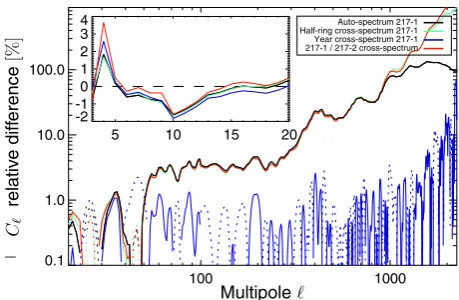
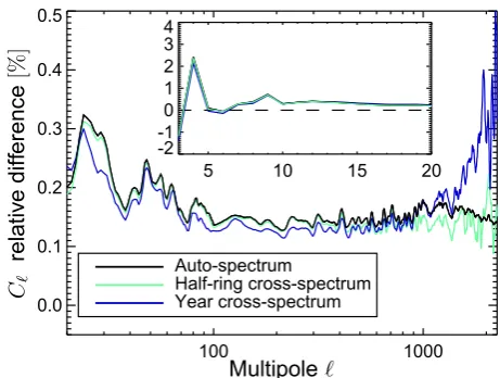
In contrast to the other lines, the 30 Hz line signal is corre-lated across bolometers (see Fig.7). It is therefore likely that the 4-K line removal procedure leaves correlated residuals on the 30 Hz line. The consequence of this correlation is that the cross-power spectra between different detectors can show ex-cess noise at multipoles around` ' 18004 (see the discussion in Sect. 1 ofPlanck Collaboration XVI 2014and in Sect. 7 of Planck Collaboration XV 2014). An example, computed with the
anafastcode in theHEALPixpackage (Górski et al. 2005), is
shown in Fig.8. To mitigate this effect, we discard all 30 Hz res-onant rings for the 16 bolometers between 100 and 353 GHz for which the median average of the 30 Hz line amplitude is above 10 aW. Doing so, the`=1800 feature disappears. This issue is also addressed in Sect. 3.1 ofPlanck Collaboration XIII(2016). Figure 9shows the fraction of discarded samples for each detector over the full mission. It gathers the flags at the sam-ple level, which are mainly due to glitches and the depointing between rings. It also shows the flags at the ring level, which are mostly due to the 4-K lines, but are also due to solar flares, big manoeuvres, and end-of-life calibration sequences, which are common to all detectors. The main difference from the nominal mission, presented in the 2013 papers, appears in the fifth survey, which is somewhat disjointed, due to solar flares arising with the increased solar activity, and to special calibration sequences. The full cold Planck-HFI mission lasted 885 days, excluding the calibration and performance verification (CPV) period of 1.5 months. During this time, HFI data losses amount to 31%, the majority of which comes from glitch flagging, as shown in Table1. The fraction of samples flagged due to solar system ob-jects (SSO), jumps, and saturation (Planck Collaboration VIII 2014) is below 0.1%, and hence negligible.
4 The spacecraft spin period of one minute implies a correspondence
-1.0 -0.5 0.0 0.5 1.0 Cross-correlation factor between the 4K line amplitudes 0
2 4 6
Normalized histogram [%]
[image:7.595.306.556.75.278.2]10 Hz line 30 Hz line
Fig. 7. Normalized histograms of the correlation coefficients of the 10 and 30 Hz 4-K line amplitudes. The amplitude is computed per ring and per bolometer from the two coefficients (sine and cosine) of a given line. For each pair of distinct bolometers (from 100 to 353 GHz), a correlation coefficient is computed between the two amplitudes during the mission. The black normalized histogram shows the 10 Hz line cor-relation coefficients of the 903 (= 43 × 42/2) pairs. The red curve shows the 30 Hz line histogram. The 30 Hz line is clearly correlated be-tween different bolometers. This is the only line that shows a significant correlation.
3.4. Detector time response
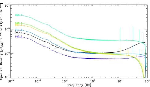
As noted in Planck Collaboration VII (2014) and Planck HFI Core Team(2011a), the detector time response is a key calibra-tion parameter for HFI. It describes the relacalibra-tion between the opti-cal signal incident on the detectors and the output of the readout electronics. This relation is characterized by a gain, and a time shift, dependent on the temporal frequency of the incoming op-tical signal. As in previous releases, it is described by a linear complex transfer function in the frequency domain, which we call the time transfer function. This time transfer function must be used to deconvolve the data in order to correct the frequency-dependent time shift, which otherwise significantly distorts the sky signal. The deconvolution also restores the frequency de-pendent gain. It is worth noting that: (i) the deconvolution sig-nificantly reduces the long tail of the scanning beam; (ii) it also symmetrizes the time response, which allows us to combine sur-veys obtained by scanning in opposite directions; and (iii) given that the gain decreases with frequency, the deconvolution boosts the noise at high frequency, as can be seen in Figs.23and26. In order to avoid unacceptably high noise in the highest temporal frequencies, a phaseless low-pass filter is applied, with the same recipe as in Sect. 2.5 ofPlanck Collaboration VII(2014). This process results in a slightly rising noise in the high frequency part of the noise power spectrum, in particular for the slowest 100 GHz detectors. This noise property is ignored in the map making process, which assumes white noise and low frequency noise. We note, however, that the 100 GHz bolometers data are not used for CMB analysis at smaller angular scales, due to their wider main beams.
For this release, the time transfer function is based on the same model as the previous release. As a function of the angular frequencyω, it is defined by
TF(ω)=F(ω)H0(ω;Sphase, τstray), (3)
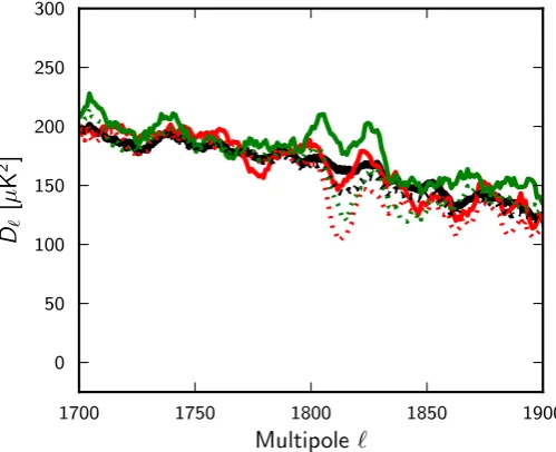
1700 1750 1800 1850 1900
Multipole
`
0 50 100 150 200 250 300
D
`[
µ
K
2
]
Fig. 8. Temperature cross power-spectrum of the 217 GHz detector sets 1 and 2 for the full mission (black) and yearly cuts (Year 1 in red and Year 2 in green), comparing the 2013 (dashed lines) and 2015 (con-tinuous lines) data release.
whereF(ω) is the term associated with the bolometer response,
and H0(ω;Sphase, τstray) is the analytic model of the
electron-ics transfer function, whose detailed equations and parameters are given in Appendix A ofPlanck Collaboration VII(2014). The electronics term depends only on two parameters: the phase shift between the AC bias current and the readout sampling, en-coded by the parameterSphase; and the time constantτstray
as-sociated with the stray capacitance of the cables connecting the bolometers to the bias capacitors (the stray capacitance enters in the h0 term in the series of filters reported in Table A.1 of
Planck Collaboration VII 2014).
The bolometer time transfer function is described by the sum of five single-pole low-pass functions, each with a time con-stantτiand an associated amplitudeai:
F(ω)= X i=1,5
ai 1+iωτi
· (4)
Fig. 9.Fraction of discarded data per bolometer (squares with black line). The fraction of data discarded from glitch flagging alone is shown with stars and the green line. The blue line with diamonds indicates the average fraction of discarded samples in valid rings. The two bolometers showing permanent random telegraphic signal (RTS), i.e. 143-8 and 545-3, are not shown, because they are not used in the data processing.
0 1 2 3 4 5
Time [s]
−10−3
−10−4
−10−05
10−5
10−4
10−3
10−2
10−1
100
Signa
l[
pea
k
units]
short glitch Jupiter
Fig. 10. Impulse response of bolometer 143-6 to short glitches and to Jupiter. The plotted axis is linear within the range±10−5 and logarithmic
elsewhere.
signal-to-noise ratio, it provides the most sensitive measurement of the longest time constants. Although the physical process of energy injection into the detector is different for microwave pho-tons and energetic particles, the heat dissipation is expected to be the same. For this reason, it was decided to take only the time constants from the glitches, and not the associated amplitudes. The impact of the incomplete correction of the transfer function is discussed in Sect.3.4.1.
In summary, the values of the bolometer time transfer func-tion parameters,aiandτi, are measured with the following logic: – the two fastest time constants, τ1 and τ2, and the
associ-ated amplitudes a1 anda2, are unchanged with respect to
the previous version, i.e., they are estimated from planet observations;
– the two longest time constants,τ4andτ5, are estimated from
short glitch stacking, together with thea5/a4ratio;
– τ3,a3, anda4 are fitted from Jupiter scans, keepingτ1,a1, τ2, anda2fixed, while the value ofa5is set to keep the same
ratioa5/a4as in the glitch data;
– a5is fitted from the CMB dipole time shift. It should be noted
that the same dipole time shift can be obtained with different combinations ofa5andτ5and for this reason,τ5is recovered
from the short glitches, and only a5 from the dipole time
shift.
This process was used for all channels from 100 to 217 GHz. For the 353 GHz detectors, different processing was needed to avoid strong non-optical asymmetries in the recovered scanning beam (see AppendixC for details). For the submillimetre channels, 545 and 857 GHz, the time transfer function is identical to that of the 2013 release. The values of the time response parameters are reported in Table C.1. The model and parameters will be improved by continuing this activity for future releases.
3.4.1. Time response errors
The beam model is built from time-ordered data deconvolved by the time transfer function. For this reason, and considering the constant rotation rate ofPlanck, the measured scanning beam absorbs, to a large extent, mismatches between the adopted time transfer function and the true one (Planck Collaboration VII 2014). In this sense, errors and uncertainties in the time trans-fer function should not be propagated into an overall window function uncertainty, since the time response acts as an error-free regularization function. Biases and uncertainties are taken into account in the beam error budget.
0.0 0.2 0.4 0.6 0.8 1.0 1.2 1.4
Time [s]
10−4 10−3 10−2 10−1 100
Signa
l[
pea
k
units]
Fig. 11. A scan across Jupiter with bolometer 143-1b, pre-deconvolution in black, post-deconvolution in red.
the constant scan rate. Simulations with varying time response parameters show that errors at frequencies above 2 Hz are ab-sorbed in the scanning beam map and propagated correctly to the effective beam window function to better than the scanning beam errors. Errors on time scales longer than 0.5 s are not absorbed by the scanning beam map, but propagate into the shifted dipole measurement and the relative calibration error budget (see Paper B).
Additionally, the time response error on time scales longer than 0.5 s can be checked by comparing the relative amplitude of the first acoustic peak of CMB anisotropies between frequency bands. The main calibration of HFI is performed with the CMB dipole (appearing in the TOI at 0.016 Hz), while the first acoustic peak at`≈200 appears at 6 Hz. Table 3 inPlanck Collaboration I(2016) shows that between 100 and 217 GHz the agreement is better than 0.3%.
3.4.2. Focal plane phase shift from fast Mars scan
In December 2011,Planckunderwent a series of HFI end-of-life tests. Among these, a speed-up test was performed increasing the spin rate to 1.4 rpm from the nominal value of 1 rpm. The test was executed on 7–16 December 2011, and included an obser-vation of Mars. Right after the test, a second Mars obserobser-vation followed, at nominal speed. The main result of this test was the ability to set the real position of the detectors in the focal plane, which, when scanning at constant speed, is completely degener-ate with a time shift between bolometer data and pointing data. This time shift was supposed to be zero. During the test, it was found that the deconvolved bolometer signals peaked at a dif-ferent sky position for the nominal scans and for the fast scans. This discrepancy was solved by introducing a time-shift between bolometer readout and pointing data. This time-shift is not the same for all detectors, and ranges from 9.5 to 12.5 ms, with a corresponding position shift ranging from 3.03 to 4.05 in the scan-ning direction. Due to time constraints, it was not possible to observe Mars twice with the full focal plane, so it was decided to favour the CMB channels and the planet was observed with all the 100, 143, 217, and 353 GHz detectors. For the other de-tectors, we used the average time-shift of all the measured detec-tors. Notably, this detector-by-detector shift resulted in a better agreement of the position in the focal plane of the two PSBs in the same horn.
Working with fast spin-rate deconvolved data is complicated by aliasing effects. For this reason the fitting procedure followed
a forward sense approach, by modelling the signal with a beam centred in the nominal position, then convolving the fast and nominal timelines with the time transfer function, and fitting the correct beam centres by comparing data and model for both fast and nominal spin-rates. For the same reason, a direct comparison of deconvolved timeline has not proven to provide better con-straints on the time-response parameters.
4. Planets and main beam description
We follow the nomenclature ofPlanck Collaboration VII(2014), where the “scanning beam” is defined as the coupled response of the optical system, the deconvolved time response function, and the software low-pass filter applied to the data. The “effective beam” represents the averaging of signal due to the scanning of the telescope and mapmaking, and varies from pixel to pixel across the sky.
Here we redefine the “main beam” to be the scanning beam out to 1000from the beam axis. The sidelobe structure at this radius is dominated by diffraction at the mirror edges and falls as∝θ−3, whereθis the angle to the main beam axis. The main
beam is used to compute the effective beam and the effective beam window function, which describes the filtering of sky signals.
The smearing of the main beam cannot be significantly re-duced without boosting the high-frequency noise. The regular-ization function (a low-pass filter) chosen has approximately the same width as the instrumental transfer function. The deconvo-lution significantly reduces the long tail of the scanning beam (see Fig.11). The deconvolution also produces a more symmet-ric time response, so residual “streaking” appears both ahead and behind the main beam, though ahead of the beam it is at a level of less than 10−4of the peak response.
The “far sidelobes” are defined as the response fromθ >5◦, roughly the minimum in the optical response. The response be-gins to rise as a function of angleθbeyond this due to spillover. The far sidelobes are handled separately from the beam effects (see Sect.4.6for justification and Paper B for details).
Table 2. Band-average scanning beam solid angle (ΩSB) and
Monte Carlo-derived errors (∆ΩMC) including noise, residual glitches,
and pointing uncertainty.
Band ΩSB ∆ΩMC
[GHz] [arcmin2]
100 . . . 104.62 0.13% 143 . . . 58.80 0.07% 217 . . . 26.92 0.13% 353 . . . 25.93 0.09% 545 . . . 25.23 0.08% 857 . . . 23.04 0.08%
– The TOI from Saturn and Jupiter observations are merged prior to B-spline decomposition, taking into account resid-ual pointing errors and variable seasonal brightness. This is achieved by determining a scaling factor and a pointing off -set by fitting the TOI to a template from a previous estimate of the scanning beams. We iterate the planet data treatment, updating the template with the reconstructed scanning beam. The process converges in five iterations to an accurcay of better than 0.1% in the effective beam window function. – Steep gradients in the signal close to the planet reduce the
completeness of the standard glitch detection and subtraction procedure, so the planet timelines are deglitched a second time.
– The beam pipeline destripes the planet data, estimating a sin-gle baseline between 3◦and 5◦before the peak for each scan-ning circle. Baseline values are smoothed with a sliding win-dow of 40 circles. The entire scanning circle is removed from the beam reconstruction if the statistic in the timeline region used to estimate the baseline is far from Gaussian.
– The main beam is now recontructed on a square grid that extends to a radius of 1000from the centroid, as opposed to 400in the 2013 data release. The cutoffof 1000was chosen so that a diffraction model of the beam at large angles from the centroid predicts that less than 5×10⁻⁵of the total solid
angle is missing.
– The scanning beam is constructed by combining data from Saturn observations, Jupiter observations, and physical op-tics models usingGRASPsoftware.
– No apodization is applied to the scanning beam map. The update of the time response deconvolved data has slightly changed the scanning beam, the effective beam solid angles, and the effective beam window functions.
4.1. Hybrid beam model
A portion of the near sidelobes was not accounted for in the effective beam window function of the 2013 data (Planck Collaboration VII 2014; Planck Collaboration XXXI 2014). To remedy this, the domain of the main beam reconstruc-tion has been extended to 1000, with no apodization. Saturn data are used where they are signal-dominated. Where the signal-to-noise ratio of the Saturn data falls below 9, azimuthally binned Jupiter data are used. At larger angles, below the noise floor of the Jupiter data, we use a power law (∝θ−3), whose expo-nent is derived fromGRASP, to extend the beam model to 1000. Figure12shows a diagram of the regions handled differently in the hybrid beam model. A summary of the solid angles of the hy-brid beams is shown in Table2. Figure13shows a contour plot
−60 −40 −20 0 20 40 60
Cross-scan [arcmin]
−60 −40 −20 0 20 40 60
Co-scan
[a
rcmin]
Diffraction model
Saturn data
Jupiter data
time response residual
−80 −70 −60 −50 −40 −30 −20 −10
peak signal [dB]
Fig. 12.Scanning beam map for detector 143-6 with a rough illustration of the regions that are handled with a different data selection or binning.
of all the scanning beams referenced to the centre of the focal plane.
4.2. Effective beams and window functions
As described inMitra et al.(2011) andPlanck Collaboration VII (2014), the FEBeCoP code is used to compute the effective beam (the scanning beam averaged over the scanning history) and theFEBeCoP andQuickbeam codes are used to compute the effective beam window functions. Statistics of the effective beams are shown in Table3.
Using Saturn and Jupiter to reconstruct the main beam in-troduces a small bias due to the large disc size of the planets as compared to Mars (see Fig. 8 of Planck Collaboration VII 2014). Additionally, Saturn’s ring system introduces a slight frequency-band dependence of the effective size of the plane-tary disc (Planck Collaboration XXXIV, in prep.). Because of Saturn’s small size relative to the HFI beams, for` <4000 the symmetric part of Saturn’s shape dominates the window func-tion. There is a small variation with HFI band in the appar-ent mean size of Saturn due to the different ring system tem-peratures, ranging from 9.0025 at 100 GHz to 10.002 at 857 GHz. Because this variation introduces a bias of less than 2 ×10⁻⁵in
B2
` for`≤4000, we ignore it and use a correction derived for a mean 9.005 Saturn disc for all bands.
The two effective-beam codes handle temperature-to-polarization leakage in slightly different ways. The dominant leakage comes from differences in the scanning beams of the polarization-sensitive detectors (see Sect.4.7). TheQuickbeam
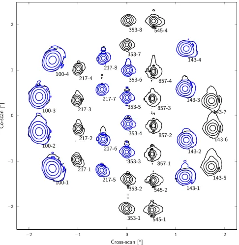
−2 −1 0 1 2
Cross-scan [
◦]
−2 −1 0 1 2
Co-sca
n
[
◦
]
100-1
100-2
100-3
100-4
143-1
143-2
143-3
143-4
143-5
143-6
143-7
217-5
217-6
217-7
217-8
217-1
217-2
217-3
217-4
353-3
353-4
353-5
353-6
353-1
353-2
353-7
353-8
545-1
545-2
545-4
857-1
857-2
857-3
[image:11.595.58.545.72.571.2]857-4
Fig. 13. B-spline hybrid scanning beams reconstructed from Mars, Saturn, and Jupiter. The beams are plotted in logarithmic contours of−3,−10,
−20, and−30 dB from the peak. PSB pairs are indicated with theabolometer in black and thebbolometer in blue.
handled later as a set of parameters in the likelihood of the angu-lar power spectra. The FEBeCoPcode produces effective beam window functions for the polarized power spectra that account for differences in the main beam. However, these are computed as the average power leakage of a given sky signal from temper-ature to polarization. Hence, these polarized window functions are not strictly instrumental parameters, since they rely on an assumed fiducial temperature angular power spectrum.
4.3. Beam error budget
As in the 2013 release, the beam error budget is based on an eigenmode decomposition of the scatter in simulated planet ob-servations. A reconstruction bias is estimated from the ensemble average of the simulations. We generate 100 simulations for each
planet observation that include pointing uncertainty, cosmic ray glitches, and the measured noise spectrum. Simulated glitches are injected into the timeline with the correct energy spectrum and rate (Planck Collaboration X 2014) and are detected and removed using the deglitch algorithm. Noise realizations are derived as shown in Sect.5.3.1. Pointing uncertainty is simu-lated by randomizing the pointing by 1.005 rms in each direction. The improved signal-to-noise ratio compared to 2013 leads to smaller error bars; for instance, at` =1000 the uncertainties onB2
` are now (2.2,0.84,0.81)×10−4for 100, 143, and 217 GHz frequency-averaged maps respectively, reduced from the previ-ous uncertainties of (61,23,20)×10−4.
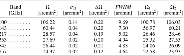
Table 3.Mean values of effective beam parameters for each HFI frequency.
Band Ω σΩ ∆Ω FWHM Ω1 Ω2
[GHz] [arcmin2] [arcmin2] [arcmin2] [arcmin] [arcmin2] [arcmin2]
100 . . . 106.22 0.14 0.20 9.69 100.78 106.03
143 . . . 60.44 0.04 0.20 7.30 56.97 60.21
217 . . . 28.57 0.04 0.19 5.02 26.46 28.46
353 . . . 27.69 0.02 0.20 4.94 25.32 27.53
545 . . . 26.44 0.02 0.21 4.83 24.06 26.09
857 . . . 24.37 0.02 0.12 4.64 22.58 23.93
Notes.The error in the solid angleσΩcomes from the scanning beam error budget. The spatial variation∆Ωis the rms variation of the solid
angle across the sky. The reported FWHM is that of the Gaussian whose solid angle is equivalent to that of the mean effective beam.Ω1andΩ2
are the solid angles contained within circles of radius 1 and 2FWHM, respectively (used for aperture photometry as described in Appendix A of Planck Collaboration XXVIII 2014).
is included in the release, for a sky fraction of 100%. Another RIMO is provided for a sky fraction of 75%. They both contain the first five beam error eigenmodes and their covariance matrix, for the multipole ranges [0, `max] with`max =2000, 3000, 3000
at 100, 143, and 217 GHz respectively (instead of 2500, 3000, 4000 previously). These new ranges bracket more closely the ones expected to be used in the likelihood analyses, and ensure a better determination of the leading modes on the customized ranges.
As described in Appendix A7 ofPlanck Collaboration XV (2014), these beam window function uncertainty eigenmodes are used to build the C(`) covariance matrix used in the high-` an-gular power spectrum likelihood analysis. It was found that the beam errors are negligible compared to the other sources of un-certainty and have no noticeable impact on the values or associ-ated errors of the cosmological parameters.
4.4. Consistency of beam reconstruction
To evaluate the accuracy and consistency of the beam recon-struction method, we have compared beams reconstructed using Mars for the main beam part instead of Saturn, and using data from Year 1 or Year 2 only. We compared the window functions obtained with these new beams to the reference ones; new Monte Carlo simulations were created to evaluate the corresponding er-ror bars, and the results are shown in Figs.14and15. Note that the effective beam window functions shown in these figures are not exactly weighted for the scan strategy, rather we plot them in the raster scan limit, where B2` is defined as the sum overm of the B2`m. The eigenmodes were evaluated for these different data sets allowing us to compare them with the reference beam using aχ2 analysis. The discrepancy between each data set and
the reference beam is fitted using Nd.o.f. = 5 eigenmodes
us-ing`max=1200, 2000, and 2500, for the 100, 143, and 217 GHz
channels, respectively. Theχ2is then defined as:
χ2=
Nd.o.f. X
i=1
(ci/λi)2 (5)
whereciis the fit coefficient for eigenvectori, with eigenvalueλi. For each data set, thep-value to exceed thisχ2value for aχ2 dis-tribution withNd.o.f.degrees of freedom is indicated in Table4.
A high p-value indicates that the given data set is consistent with the reference beam within the simulation-determined error eigenvectors, with 100% indicating perfect agreement.
We find excellent agreement between the yearly and nominal beams for the SWB bolometer channels. However, in order to
Table 4.P-values in percent for theχ2comparison of the nominal beam
with Year 1 and Year 2 data sets, following the definition in Eq. (5).
Band Year 1 Year 2
100-ds1 . . . 66.95 92.44 100-ds2 . . . 85.12 75.99 143-ds1 . . . 72.24 99.83 143-ds2 . . . 1.14 16.81 143-5 . . . 94.88 97.57 143-6 . . . 96.14 98.78 143-7 . . . 93.78 95.67 217-ds1 . . . 78.12 69.74 217-ds2 . . . 27.33 30.87 217-4 . . . 95.99 68.44 217-1 . . . 99.08 97.49 217-2 . . . 97.18 98.86 217-3 . . . 97.59 99.07
obtain reasonable beam agreement for the PSB detector sets, we find that the yearly beam errors must be scaled by a factor of 4. We conclude that there is an unknown systematic error in the beam reconstruction that is not accounted for in the simulations used to estimate the Monte Carlo error bars. We assign a scaling factor of 4 to the error eigenmodes to account for this systematic uncertainty. The additional error scaling has a negligible effect on the cosmological parameters.
4.5. Colour correction of the beam shape
In general, the measured beam shape is a function of the spectral energy distribution (SED) of the measurement source. This is of particular concern, because we measure the beam on a source with a roughly Rayleigh-Jeans SED, yet we use the effective beam window function to correct the CMB.
[image:12.595.368.497.290.441.2]−1. 0 0. 0 1.0 1500 3000 100-ds1 −1. 0 0. 0 1.0 1500 3000 100-ds2 −1. 0 0. 0 1.0 1500 3000 143-ds1 −1. 0 0. 0 1.0 1500 3000 143-ds2 −1. 0 0. 0 1.0 1500 3000 143-5 −1. 0 0. 0 1.0 1500 3000 143-6 −1. 0 0. 0 1.0 1500 3000 143-7 −1. 0 0. 0 1.0 1500 3000 217-ds1 −1. 0 0. 0 1.0 1500 3000 217-ds2 −1. 0 0. 0 1.0 1500 3000 217-4 −1. 0 0. 0 1.0 1500 3000 217-1 −1. 0 0. 0 1.0 1500 3000 217-2 −1. 0 0. 0 1.0 1500 3000 217-3 Year 1 Year 2 Full mission Multipole Multipole Multipole Multipole Multipole Multipole Multipole Multipole Multipole Multipole Multipole Multipole Multipole
W/WF ull−1 [%] 1σ
[image:13.595.42.554.80.290.2]3σ
Fig. 14.Comparison of Year 1 and Year 2 based beams with the reference beam (Full Mission). Window functions are calculated usingQuickbeam in raster scan configuration. Error bars are computed using MC simulations for Year 1 and Year 2, taking the maximal one for each.
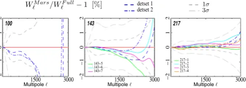
− 2 − 1 01 2 1500 3000 100 − 2 − 1 01 2 1500 3000 143 143−5 143−6 143−7 − 2 − 1 01 2 1500 3000 217 217−1 217−2 217−3 217−4 detset 1 detset 2 Multipole Multipole Multipole WMars
/WF ull−1 [%] 13σσ
Fig. 15. Comparison of Mars-based beams with the reference beam (Full Mission). Mars-based beams are constructed from Mars data for the main beam (<∼100
) and Saturn and Jupiter data for the larger scales. Window functions are calculated usingQuickbeamin raster scan con-figuration. Error bars are computed using MC simulations for Mars.
We search for a possible signature of the colour-correction effect in the data. First, we check for consistency in the CMB angular power spectra derived from different detectors and fre-quency bands using the SMICAalgorithm, in order to find dis-crepancies in beam shape and relative calibration of different data subsets using the CMB anisotropies (Planck Collaboration XI 2016). There are hints of differences that are orthogonal to the beam error eigenmodes and appear as changes in relative calibra-tion, but the preferred changes are at the 0.1% level. Because this correction is of the same order of magnitude as the relative cali-bration uncertainty between detectors, we treat it as insignificant. Second, we look at the relative calibration between detectors within a band for compact sources as a function of the source SED. In this method, any discrepancies due to solid angle vari-ation with SED are degenerate with an error in the underlying bandpass. Additionally, because of the lack of bright, compact sources with red spectra, this method is limited in its signal-to-noise ratio. In the limit that any detected discrepancy is com-pletely due to solid-angle variation with colour, at the level of 1% in solid angle we do not detect variations consistent with the physical optics predictions.
Given the lack of measurement of this effect at the current levels of uncertainty, as well as uncertainties in the modelling of the telescope, we note that this effect may be present at a small
level in the data, but we do not attempt to correct for it or include it in the error budget.
4.6. Effective beam window function at large angular scales
The main beam derived from planet observations and GRASP
modelling extends 1000 from the beam axis, so the effective beam window function does not correct the filtering of the sky signal on larger scales (approximately multipoles` < 50). In practice, due to reflector and baffle spillover, the optical re-sponse of HFI extends across the entire sky (Tauber et al. 2010; Planck Collaboration XIV 2014). According to GRASP
calculations, the far-sidelobe pattern (FSL) further than 5◦from the beam centroid constitutes between 0.05% and 0.3% of the total solid angle. To first order, this is entirely described by a correction to the calibration for angular scales smaller than the dipole (Planck Collaboration XXXI 2014).
More correctly, the far-sidelobe beam (defined here as the optical response more than 5◦from the beam axis) filters large-angular-scale sky signals in a way that is coupled with the scan history of the spacecraft, and given a perfect measurement of the far-sidelobe beam shape, an effective beam window func-tion could be constructed for the large angular scale with the same procedures used for the main beam’s effective beam win-dow function.
We rely entirely on GRASP calculations to determine the large-scale response of the instrument. These calculations are fit-ted to survey difference maps (see Planck Collaboration XXXIV, in prep.), where the single free parameter is the amplitude of the
GRASPfar-sidelobe model beam. Because of a combination of
the low signal-to-noise ratio of the data and uncertainty in the
GRASPmodel, the errors on the fitted amplitude are of the
[image:13.595.41.292.337.427.2]0.00
0.05
0.10
100
×
∆
B
`/
B
`100 GHz
143 GHz
100 101 102
Multipole
`
0.00
0.05
0.10
100
×
∆
B
`/
B
`217 GHz
100 101 102
Multipole
`
[image:14.595.40.290.73.277.2]353 GHz
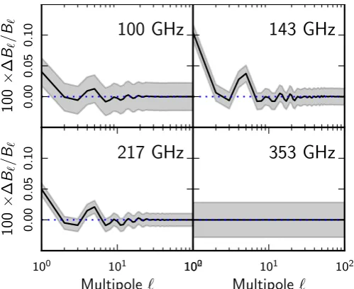
Fig. 16. Estimate of the effective beam window function corrections due to far-sidelobe response (more than 5◦
from the beam axis). Shading indicates±1σerrors. The curves in the 353 GHz panel are divided by a factor of 10; for this frequency the far sidelobe response amplitude is very low compared to the estimated errors.
Figure16shows the correction to the effective beam window function due to the best-fit far-sidelobe model. The error bars are from the amplitude error in the fit Planck Collaboration XXXIV (in prep.) and they show that the uncertainty is larger than the predicted beam window function correction except at the dipole scales (`=1), aside from a marginally significant, but negligibly small, bump at` =5. The filtering of the CMB signal with the far-sidelobe beam is thus insignificant and can be ignored as a component of the effective beam window function. A map-level correction of Galactic contamination pickup in the far-sidelobes is more appropriate. However, given the large uncertainties in the far-sidelobe model shape, we choose to neglect this correction, and note that residuals from Galactic pickup may be present in the map. The only far sidelobe effect that is corrected in the data is an overall calibration correction, as described in Paper B.
4.7. Cross-polar response and temperature-to-polarization leakage
The data model used for the HFI polarization reconstruction assumes that the entire cross-polar response of each PSB is due to the detector itself, and so the beam shape of the cross-polar response is exactly the same as the co-cross-polar beam shape. The corrugated feed horns exhibit some internal cross-polar response (Maffei et al. 2010). GRASP simulations show that this cross-polar response is at the level of 0.1–0.5%, con-siderably smaller than the detector cross-polar response (2– 5%). Simulations usingFEBeCoPshow that the effect of ignor-ing the cross-polar optical beam shape results in a smoothignor-ing of polarization power spectra equivalent to an additional 10– 2000 Gaussian, which we neglect. Additionally the data model assumes identical beams for every PSB used to reconstruct the polarization; this creates some temperature-to-polarization leak-age. Main-beam leakage dominates over the differential time re-sponse tails. Figure17shows a simulation of CMB temperature leakage into polarization power spectra using FEBeCoP, given the measured scanning beams within a band.
5. Validation and consistency tests
Here we describe some of the tests that have been done to vali-date the quality of the cleaned TOI. Other tests at the map level are described in Paper B. First we discuss the impact of the ADC correction. Then we analyse how each step of the TOI pro-cessing pipeline can alter the resulting power spectra and also study the noise properties. Finally we estimate the filtering func-tion of the TOI pipeline with end-to-end simulafunc-tions.
5.1. ADC residuals
5.1.1. Gain consistency at ring level
Using the undeconvolved TOI at the ring level, we can monitor the quality of the ADC correction with respect to the stability of the gain. For that purpose we can measure the relative gain of parity plus (g+) and parity minus (g−) samples (alternating sam-ples). The two parities sample a very different part of the ADC scale, so that a gain mismatch is a diagnostic of the ADC nonlin-earity correction. During a ring, the sky signal from both parities should be almost identical. We thus correlate a phase-binned ring (PBR) made of parity plus with the average PBR (made of both parities) and obtaing+. We similarly obtaing−. The gain half-difference (g+−g−)/2 is shown as a function of the ring num-ber in Fig.18for a representative selection of four bolometers. The improvement obtained with ADC correction is significant with a root-mean-square dispersion decreasing by a factor of 2 to 3. Only a handful of bolometers show some discrepancies at the 10−3level after the ADC correction, namely 143-3b, 217-5b,
217-7a, 217-8a, and 353-3a. This internal consistency test at the ring level is not sensitive to gain errors common to both parities. However, it agrees qualitatively with the overallBogopixgain variations shown in Paper B.
5.1.2. Parity map spectra
Two independent sky maps are produced from the two TOI pari-ties; the differences between these are again expected to capture the ADC residual effects. Figure 19compares full-sky spectra derived from maps built on raw and ADC-corrected data. Glitch-flagged samples have been removed. The behaviour in 1/`2 at low`is similar to the behaviour of simulated data as shown in Sect.2.5.
These low-`residuals, although much improved with respect to the 2013 delivery, are not yet fully under control. At the time of the 2015 delivery, work is continung to estimate how this ef-fect propagates into the cross-polarization spectra, and to give a coherent description of the different low-` systematics still present in HFI 2015 data. For this reason, among others, it has been decided to postpone the release of HFI low`polarized data.
5.2. Filtering effects
It is customary to evaluate the effects produced by the pipeline on the signal as a filtering function, depending on the considered angular scale. Here we evaluate whether or how each pipeline module (see Fig.1) filters the signal.
– ADC correction. The ADC nonlinearities add a spurious component to the power spectra. Correcting for it removes this component, reducing theC`by an amount smaller than 1%, that depends on the channel, and is very flat in`. – Glitch removal/flagging. Using simulations, Planck
Fig. 17. A simulation of the ratio of temperature-to-polarization leakage, given the main beam mismatch, compared toEEandBBsignal.
[image:15.595.37.557.332.716.2]